
Long-Term Performance of Energy
Efficiency Loan Portfolios
March 2022
DOE/EE-2561

March 2022 www.seeaction.energy.gov ii
Lo
ng-Term Performance of Energy Efficiency Loan Portfolios was developed as a product of the State and Local
Energy Efficiency Action Network (SEE Action), facilitated by the U.S. Department of Energy and the U.S.
Environmental Protection Agency. Content does not imply an endorsement by the individuals or organizations that
are part of SEE Action working groups, or reflect the views, policies, or otherwise of the federal government.
This document was final as of March 2022.
If this document is referenced, it should be cited as:
State and Local Energy Efficiency Action Network (SEE Action). (2021). Long-Term Performance of Energy Efficiency
Loan Portfolios. Prepared by: Jeff Deason, Greg Leventis, and Sean Murphy of Lawrence Berkeley National
Laboratory.
FOR MORE INFORMATION
Regarding Long-Term Performance of Energy Efficiency Loan Portfolios, please contact:
Jeff Deason Greg Leventis
Berkeley Lab Berkeley Lab
JADeason@lbl.gov [email protected]
Regarding the State and Local Energy Efficiency Action Network, please contact:
Johanna Zetterberg
U.S. Department of Energy
March 2022 www.seeaction.energy.gov iii
Acknowledgments
The work described in this study was funded by the U.S. Department of Energy’s Office of Weatherization and
Intergovernmental Programs and the Office of Strategic Analysis under Lawrence Berkeley National Laboratory
Contract No. DE-AC02-05CH11231.
The authors would like to thank Emily Basham (Connecticut Green Bank), Joe Buonannata (Inclusive Prosperity
Capital), Peter Krajsa (National Energy Improvement Fund), Kerry O’Neill (Inclusive Prosperity Capital), Todd Parker
(Michigan Saves), Jeff Pitkin (NYSERDA), and Mary Templeton (Michigan Saves) for their contributions to this
report. The authors would also like to thank the U.S. Department of Energy’s Johanna Zetterberg, Sean Williamson,
and Ookie Ma for their guidance and input.
This report was reviewed by: Neda Arabshahi (Inclusiv), Dana Clark (Nutmeg State Financial Credit Union), Brian
Ford (KBRA), Anna Maria Garcia (Department of Energy), Lain Gutierrez (CleanFund), Eric Hangen (University of
New Hampshire), Bert Hunter (Connecticut Green Bank), Peter Krajsa (National Energy Improvement Fund), Ookie
Ma (Department of Energy), Eddie McRoberts (OmniCap), Eric Neglia (KBRA), Kerry O’Neill (Inclusive Prosperity
Capital), Jeff Pitkin (NYSERDA), Al Quintero (Ramirez), Valerie Schuette (True CCU), Jeff Smith (OmniCap), Mary
Templeton (Michigan Saves), Cal Vinal (Capital for Change), Keith Welks (Pennsylvania Treasury), and Sean
Williamson (Department of Energy).
The authors would like to give a special thank you to Bryan Garcia (Connecticut Green Bank) and Bruce Schlein
(OMERS Infrastructure Management Inc), and the State and Local Energy Efficiency Action Network’s Financing
Solutions Working Group, who helped conceptualize and guide this project.
Disclaimer
This document was prepared as an account of work sponsored by the United States Government. While this
document is believed to contain correct information, neither the United States Government nor any agency
thereof, nor The Regents of the University of California, nor any of their employees, makes any warranty, express
or implied, or assumes any legal responsibility for the accuracy, completeness, or usefulness of any information,
apparatus, product, or process disclosed, or represents that its use would not infringe privately owned rights.
Reference herein to any specific commercial product, process, or service by its trade name, trademark,
manufacturer, or otherwise, does not necessarily constitute or imply its endorsement, recommendation, or
favoring by the United States Government or any agency thereof, or The Regents of the University of California.
The views and opinions of authors expressed herein do not necessarily state or reflect those of the United States
Government or any agency thereof, or The Regents of the University of California.
Ernest Orlando Lawrence Berkeley National Laboratory is an equal opportunity employer.
Copyright Notice
This manuscript has been authored by an author at Lawrence Berkeley National Laboratory under Contract No. DE-
AC02-05CH11231 with the U.S. Department of Energy. The U.S. Government retains, and the publisher, by
accepting the article for publication, acknowledges, that the U.S. Government retains a non-exclusive, paid-up,
irrevocable, worldwide license to publish or reproduce the published form of this manuscript, or allow others to do
so, for U.S. Government purposes.
March 2022 www.seeaction.energy.gov iv
Table of Contents
Acknowledgments ............................................................................................................................................. iii
Disclaimer .......................................................................................................................................................... iii
Copyright Notice ................................................................................................................................................ iii
List of Figures ...................................................................................................................................................... v
List of Tables ...................................................................................................................................................... vi
Executive Summary .........................................................................................................................................ES-1
Loan and borrower characteristics ...................................................................................................................ES-1
Loan performance ............................................................................................................................................ ES-1
Performance compared to other financial products ........................................................................................ES-2
1. Introduction .............................................................................................................................................. 1
2. Studied energy efficiency loan portfolios ................................................................................................... 1
2.1. Program overviews ..................................................................................................................................... 2
2.2. Descriptive statistics ................................................................................................................................... 4
2.2.1. Loan characteristics ...................................................................................................................... 4
2.2.2. Borrower characteristics .............................................................................................................. 8
3. Performance analysis ............................................................................................................................... 11
3.1. Methodology ............................................................................................................................................ 11
3.2. Findings ..................................................................................................................................................... 12
3.2.1. Delinquency and loss analysis .................................................................................................... 12
3.2.2. Prepayment ................................................................................................................................ 18
3.2.3. Regression analysis ..................................................................................................................... 18
4. Comparators ............................................................................................................................................ 20
4.1. Methodology ............................................................................................................................................ 20
4.2. Findings ..................................................................................................................................................... 22
5. Conclusions .............................................................................................................................................. 24
6. Areas for future work ............................................................................................................................... 25
References ........................................................................................................................................................ 27
Appendix A: Regression results ....................................................................................................................... A-1
Appendix B: Participation by CRA income bin ................................................................................................ 2B-1

March 2022 www.seeaction.energy.gov v
List of Figures
Figure ES1. Delinquency rates, energy efficiency loans and comparators ............................................................... ES-2
Figure 1. Loan volumes by program and vintage ........................................................................................................... 2
Figure 2. Participation by principal amount bin ............................................................................................................ 4
Figure 3. Participation by monthly payment amount .................................................................................................6
Figure 4. Share of portfolio participants with different loan terms .............................................................................. 7
Figure 5. Participation by interest rate .......................................................................................................................... 8
Figure 6. Participant incomes (by AMI bin) for three portfolios .................................................................................. 10
Figure 7. Participation in four efficiency financing programs by credit score bin ....................................................... 11
Figure 8. Delinquency rates by program ..................................................................................................................... 13
Figure 9. Cumulative gross loss rates by program and years of seasoning ................................................................. 14
Figure 10. Delinquency (share of outstanding loans) by credit score bin ................................................................... 15
Figure 11. Cumulative gross loss by credit score bin ................................................................................................... 15
Figure 13. Cumulative gross loss rates by AMI band ................................................................................................... 17
Figure 14. Delinquency rates, energy efficiency loans and comparators .................................................................... 22
Figure 15. Cumulative loss rates for, energy efficiency loans (gross) and KBRA Prime Auto (net) and Tier 1
Consumer Loans (net) .................................................................................................................................................. 23
Figure 16. Annualized loss rates, EE loans and comparators ...................................................................................... 24
Figure 17. Participation by CRA income bin .............................................................................................................. B-1
Figure 12. Delinquency (share of outstanding loans) by program and AMI band........................................................ 16

March 2022 www.seeaction.energy.gov vi
List of Tables
Table 1. Description of the loan portfolios studied ....................................................................................................... 2
Table 2. Program portfolios included in this analysis .................................................................................................... 3
Table 3. Average and median principal amounts, monthly payments, terms, and interest rates ................................ 5
Table 4. Average and median borrower characteristics ................................................................................................ 9
Table A-1. Regression output for all loan portfolios combined (n=51,041) .............................................................. A-1
Table A-2. Regression output for all loan portfolios with income (n+36,288) .......................................................... A-1
Table A-3. Regression output for Michigan Saves (n=14,905) ................................................................................... A-2
Table A-4. Regression output for CT Smart-E (n=3,166) ............................................................................................ A-2
Table A-5. Regression output for Keystone HELP (n=14,753) .................................................................................... A-3
Table A-6. Regression output for NYSERDA Smart Energy (n=14,176) ...................................................................... A-3
Table A-7. Regression output for NYSERDA On-Bill Recovery (n=3,849) ................................................................... A-4

March 2022 www.seeaction.energy.gov ES-1
Executive Summary
This report reviews and documents the financial performance of four large and long-running residential energy
efficiency financing programs. The analysis presented will inform potential capital providers, lenders, and program
administrators and help them assess the likely outcomes and risks associated with energy efficiency lending.
Anecdotally, performance of energy efficiency lending is generally understood to be strong, but data on energy
efficiency loan performance has not been readily available. The data made available in this report significantly
expand the public evidence base.
This report reviews loan performance data from four programs:
• The Connecticut Green Bank (CGB)’s Smart-E Loan program, which began issuing loans in 2013;
• The Keystone HELP program run through the Pennsylvania Treasury, which began issuing loans in 2006;
• The Michigan Saves loan program, which began issuing loans in 2010; and
• The New York State Energy Research and Development Agency (NYSERDA)’s loan programs, which began
issuing loans in 2010.
Loan and borrower characteristics
The average loan across the four studied portfolios (52,511 energy efficiency-only loans) has the following
characteristics:
• A principal amount of $9,137;
• A loan term of 121 months (just over ten years);
• An average seasoning (i.e., time since a loan was issued) of 4.5 years;
• An interest rate of 5.0%;
• A monthly payment amount of $93; and
• Is unsecured.
1
While there is some variation across programs, in general the loans are relatively similar along these parameters.
Borrowers in these programs have relatively high credit scores, concentrated in the 660-780 range with an average
of 740. The average borrower lives in a census tract with a median household income between 80% and 100% of
the median income in its metropolitan statistical area. Borrower characteristics are also comparable across the
four programs.
Loan performance
Our data document each pool’s delinquency and loss status as of a specific date (March 2020 for NYSERDA and
Smart-E, December 2019 for Michigan Saves, and September 2017 for Keystone HELP). Across the four portfolios:
• The 30-day delinquency rate – the share of outstanding loan dollars that are at least 30 days delinquent –
is 1.57% (the 60-day delinquency rates is 0.62%, and the 90-day delinquency rate is 0.21%).
1
In some on-bill lending programs (including both Michigan Saves’ and NYSERDA’s on-bill programs), nonpayment could result in disconnection
of the participant’s power service. Although some may refer to disconnection as “security” for these loans since it could incentivize repayment,
technically secured loans carry the potential loss of some form of collateral (e.g., a car or a home); this both incentivizes repayment and also
helps to make the lender whole in case of a loss. Disconnection would not help make a lender whole after a loss. On-bill loans comprise only a
small subset of the loans in the portfolios.
March 2022 www.seeaction.energy.gov ES-2
• Losses (charge offs) are highest early in loan lifetimes and decline later, a common finding for consumer
loans. The pooled portfolios lost 2.1% of the principal by year 2, 3.3% by year 4, 4.5% by year 6, and 5.1%
by year 8.
Regression analysis identifies features of loans and borrowers that are associated with strong loan performance:
• Borrower credit scores stand out: all else equal (e.g., same interest rate, loan age, and borrower income),
increasing borrower credit score by 100 lowers the odds that a given loan is 30 days delinquent by 1.06
percentage points and the odds that a given loan is charged off by 5.81 percentage points.
• Income metrics (the income of the census tract in which the borrower lives, as well as household income
available for one portfolio) are also associated with loan performance; however, this association is not
nearly as strong as that with credit score, demonstrating that credit score is a better predictor of loan
performance than income.
Performance compared to other financial products
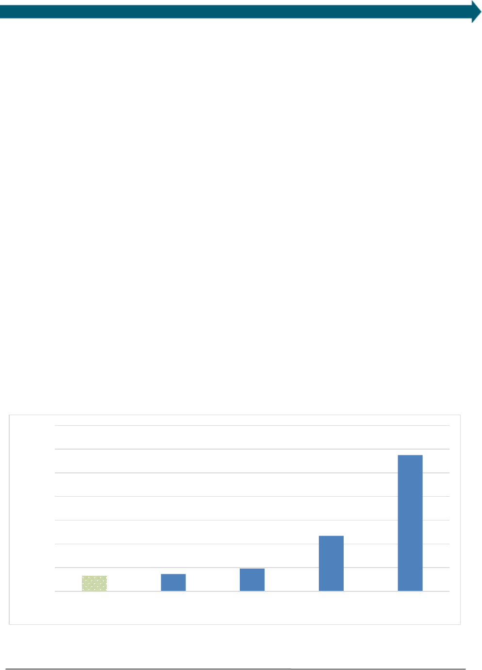
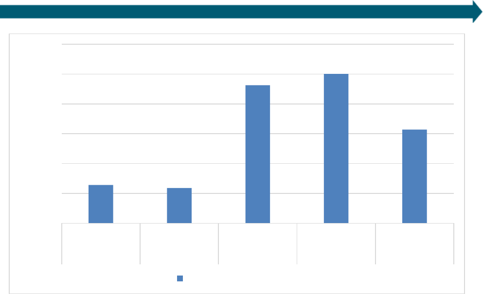
The delinquency and loss rates of loans in the studied energy efficiency loan portfolios are low compared with
unsecured consumer loans and are comparable to the rates for prime auto loans, which are secured by the
vehicles (see Figure ES1). This strong performance may be supported by utility bill savings resulting from the
financed efficiency projects or also may in part reflect differences in borrower and loan characteristics between
the efficiency loans and comparators. Regardless, the data provide the most comprehensive evidence to date that
lenders and capital providers can expect energy efficiency loans—at least those from well-designed and
administered programs such as those studied here— to perform well.
These findings show that financial institutions can market energy efficiency improvements to their customers and
lend them the money they need for those projects at low risk, while creating a more efficient building stock. The
data show that households from low- and moderate-income areas participate in these programs and that high-
credit borrowers in these areas repay at a strong rate, suggesting efficiency financing could support policy goals
related to equitable access (e.g., Justice 40 goals and Community Reinvestment Act compliance requirements).
This analysis can inform the design of credit enhancement mechanisms, such as loan loss reserves, at the federal
or state level—for example, by setting loan performance expectations to help size financial outlays — that could
help encourage financial institutions to increase energy efficiency lending.
Figure ES1. Delinquency rates, energy efficiency loans, and comparators
0%
1%
2%
3%
4%
5%
6%
7%
Pooled EE loans, all
programs
Auto loans, prime
only (KBRA)
Non-credit card cons
loans (Fed)
Consumer loans, with
credit (Fed)
Tier 1 consumer loans
(KBRA)
Annualized Gross Loss Rates

March 2022 www.seeaction.energy.gov 1
1. Introduction
This report presents a detailed analysis of energy efficiency loan performance data from four large and long-
running residential programs. Although smaller-scale energy efficiency financing programs have operated for many
years, several larger programs were operating by 2010. These programs have now accrued enough historical data
to be of sufficient volume and maturity for substantive analysis.
Energy efficiency stakeholders have long theorized that borrowers in energy efficiency loan programs may have
low delinquency and loss rates. These loans might perform strongly because the projects being financed reduce
energy consumption and save borrowers money, leaving them with additional resources to repay the loans.
Another explanation may be because the types of households that participate in these programs may be low risk in
ways that traditional loan underwriting may not capture. For example, these households are investing in their
properties, thereby demonstrating that they value them, and are identifying and pursuing relatively small savings
opportunities, thereby demonstrating their careful attention to their expenditures (Zimring et al. 2013). The
analysis presented here is a first step toward testing this theory.
Capital market stakeholders are generally unfamiliar with energy efficiency loans.
2
Prior to this report, no
comprehensive, loan-level analyses of the financial performance of energy efficiency loans were publicly available.
If lenders and capital providers lack data regarding the true risks of these loans, they may ration credit (Palmer et
al. 2012), offering less desirable terms than they would if they had better information. This report provides
investors, lenders, and program administrators with data regarding the attributes of energy efficiency loans and
their performance.
Section 2 reviews the four energy efficiency programs studied and presents a detailed description of the loan
portfolios. Section 3 reviews the performance of these portfolios in terms of delinquency rates, charge-off rates,
and prepayment. Section 4 compares their performance to that of other financing asset classes to put the report’s
findings in context. Section 5 concludes.
2. Studied energy efficiency loan portfolios
Berkeley Lab obtained loan-level data for four residential energy efficiency financing portfolios: Keystone HELP,
Michigan Saves, the New York State Energy Research and Development Authority’s (NYSERDA) On-bill Recovery
Loan and Smart Energy Loan programs, and the Connecticut Green Bank’s Smart-E Loan program.
All of these programs except for Keystone HELP make loans for both energy efficiency and solar projects. Because
this report addresses loans for energy efficiency, loans that included solar PV were excluded. Furthermore, loans
made for the two technologies may not perform comparably. Berkeley Lab will address the performance of solar
loans in these portfolios in future work.
In total, the data include 52,511 loans. Due to occasional missing data, some data elements presented in this
report have fewer observations.
For three of the portfolios, Berkeley Lab was able to obtain data from program inception through the end of 2019
or beginning of 2020 (see Table 1 for specific dates for each portfolio). Notably, all data sets end before the
financial impacts of the Covid-19 pandemic began.
2
This differentiates energy efficiency loans from solar loans, which are more established in securities markets.
March 2022 www.seeaction.energy.gov 2
Table 1. Description of the loan portfolios studied
Program
State
Years of data
Total non-PV loans
Keystone HELP
PA
February 2006—September 2017
14,753
Michigan Saves
MI
October 2010—December 2019
16,042
NYSERDA
NY
December 2010—March 2020
18,556
Smart-E
CT
May 2013—March 2020
3,160
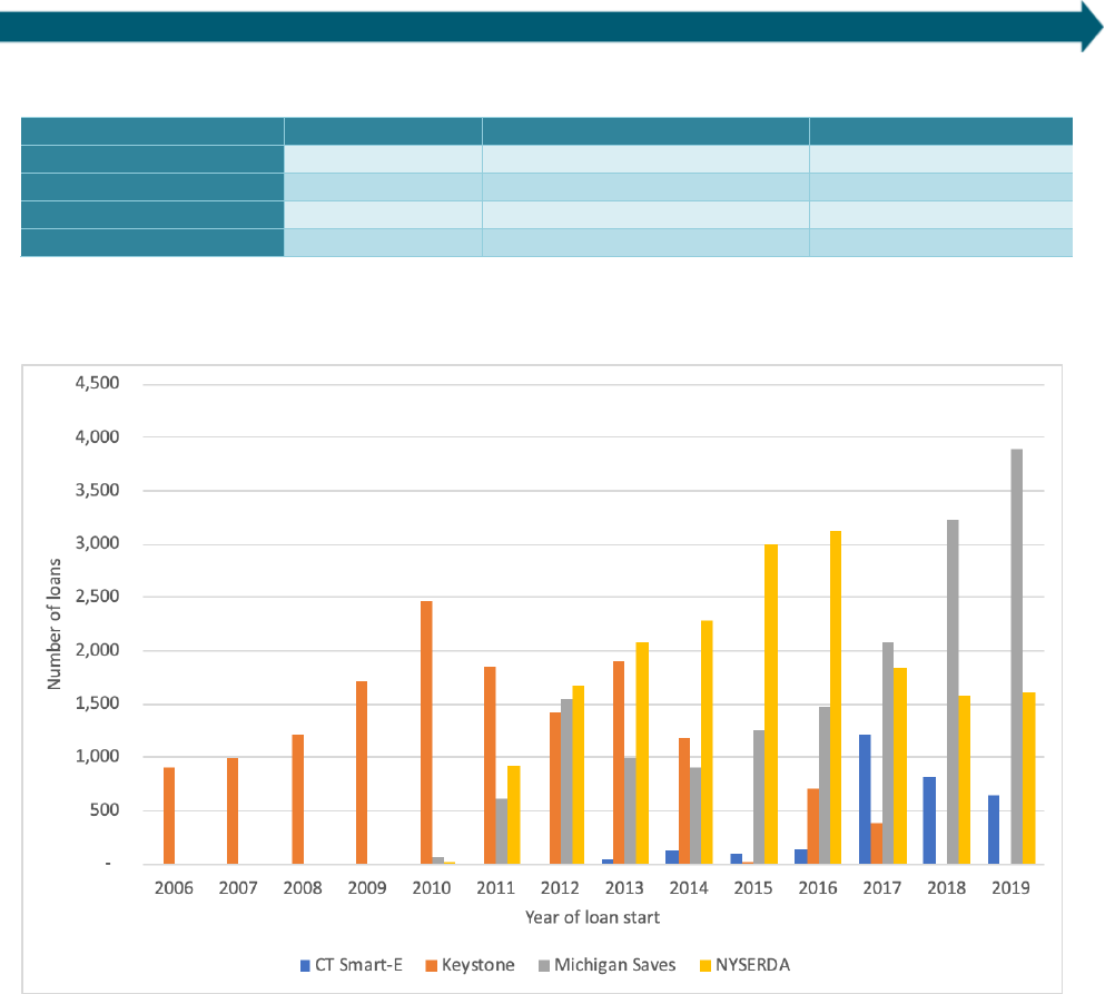
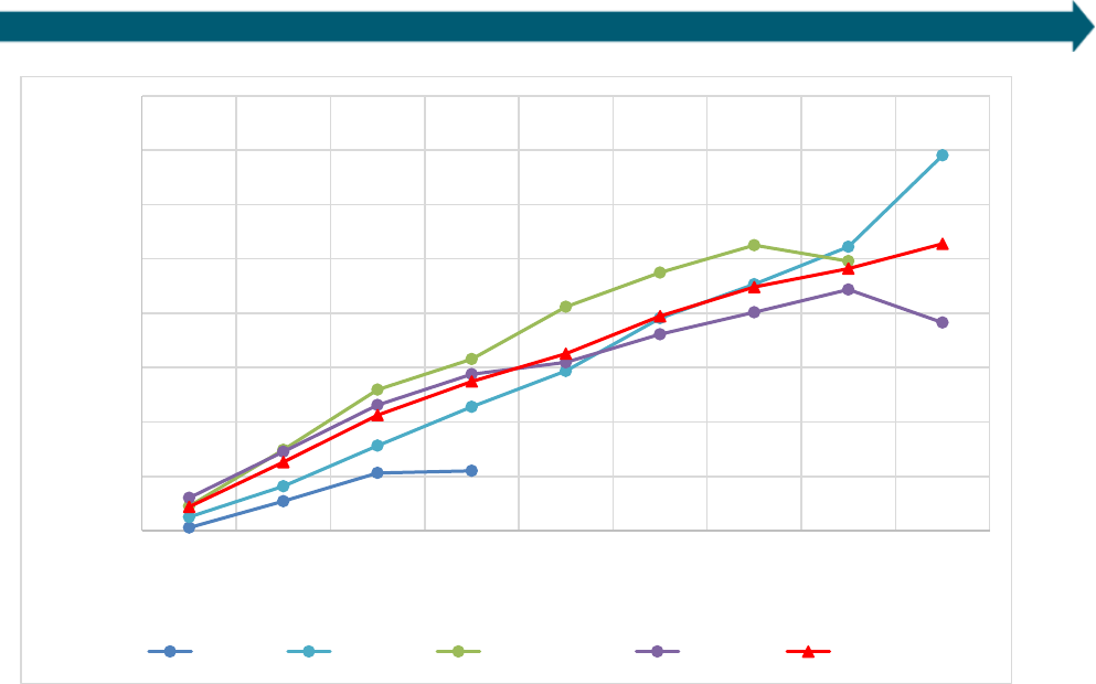
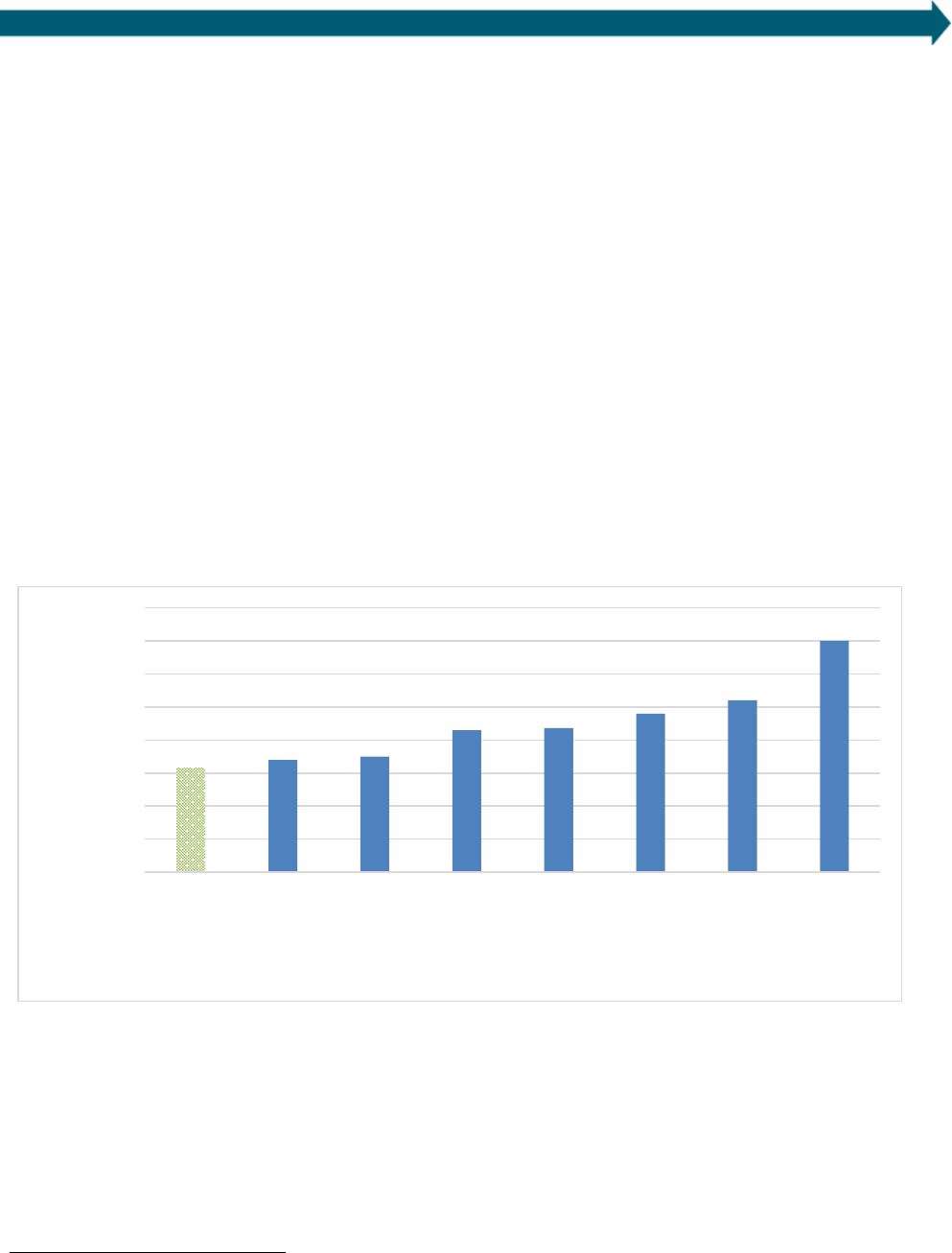
Fi
gure 1 shows the different program volumes by vintage, i.e., the year in which each loan was made.
F
igure 1. Loan volumes by program and vintage
For Keystone HELP, data were only available on loan status as of September 2017. Since this program began in
2006, this still represents 11 years of program loans. Keystone HELP is also the one program analyzed with
significant activity prior to the 2008 recession, and thus has navigated an economic cycle. The other programs
began after the recession. The Michigan Saves and Smart-E programs made the bulk of their loans in the last three
years of the analysis period.
2.1. Program overviews
The loan portfolios included in the analysis come from four energy efficiency loan programs: the Connecticut
Green Bank’s Smart-E Loan program, Pennsylvania’s Keystone HELP program, Michigan Saves’ programs, and the
Green Jobs, Green New York programs (comprised of the On-bill Recovery Loan and Smart Energy Loan) of the
New York State Energy & Research Development Authority (NYSERDA). See Table 2.
March 2022 www.seeaction.energy.gov 3
T
able 2. Program portfolios included in this analysis
Program
Smart-E
Keystone HELP
Michigan Saves
Green Jobs Green New York
Program administrator (PA)
Connecticut Green Bank (CGB) and Inclusive
Prosperity Capital (IPC)
AFC First
a
Michigan Saves
NYSERDA
Description of PA
Quasi-governmental green bank increasing flow
of private capital to markets that energize the
green economy
Private energy efficiency financing
company
Nonprofit green bank funding
clean energy
State authority advancing clean energy
innovation and investments
Lender (entity extending program
loans)
13 local financial institutions
b
AFC First
a
7 local financial institutions
b
NYSERDA
Underwriting criteria
CGB/IPC ask lenders to use their standard
practice: FICO (min. 640 or 580), Debt-to-
income (DTI) (max. 50% or 45%), no bankruptcy
in last 4 to 7 years, income verification
c
Min. credit 640
Max. DTI 50% (42% for loans >$25K), no
bankruptcy for 5 years
Min. credit 600
Max. DTI 50%, no bankruptcy for
12 months; for on-bill, 12 months
on-time utility bill payment
Min. credit score 540
Max. DTI depends on credit score, no
bankruptcy for 2 years, 12 months on
time mortgage payments
Loan underwriter
13 local financial institutions
b
AFC First
a
7 local financial institutions
b
Slipstream
Structure (on- vs off-bill, secured
d
or unsecured)
Unsecured, off-bill loans
Unsecured, off-bill loans
Unsecured, on- and off-bill loans
Unsecured, on- and off-bill loans
Credit enhancements (CE) to
lenders (does not include CEs for
secondary market loan sales)
Loan loss reserve (second loss, at the portfolio
level)
Loss reserves were provided through
various Pennsylvania state agencies and
grants
Loan loss reserve, and utility
capital from one publicly-owned
utility
None
Source of capital
Local financial institutions
Pennsylvania Treasury, AFC First,
securitization proceeds, local bank loan
pool
Local financial institutions,
municipal utility capital (for
Holland on-bill program)
Regional Greenhouse Gas Initiative
funds
e
, securitization proceeds
Federal funds used
American Recovery and Reinvestment Act
(ARRA) funds for loan loss reserve and interest
rate buydowns at different points in the
program
ARRA funds provided loss reserves and
rate buydown funds for some of the
program years
ARRA funds provided the loan loss
reserve
None
a
The program administration changed in 2015 upon AFC First’s acquisition by Renew Financial. AFC First was also lender and underwriter for the program. The National Energy
Improvement Fund (NEIF), a successor run by AFC First’s management, is now providing administration services for a portion of the portfolio.
b
For residential program participants.
c
Participating lenders can use standard or credit-challenged term sheets; underwriting thresholds depend on which is used.
d
In some on-bill lending programs (including both Michigan Saves’ and NYSERDA’s on-bill programs), nonpayment could result in disconnection of the participant’s power service.
Although some may refer to disconnection as “security” for these loans since it could incentivize repayment, technically secured loans carry the potential loss of some form of collateral
(e.g., a car or a home); this both incentivizes repayment and also helps to make the lender whole in case of a loss. Disconnection would not help make a lender whole after a loss.
e
See: https://www.rggi.org.
March 2022 www.seeaction.energy.gov 4
2.2. Descriptive statistics
This section describes several characteristics of the studied efficiency loan program portfolios: four properties of
the loans themselves (loan tenors, principal amounts, monthly payment amounts, and interest rates) and two
characteristics of the participants (incomes and credit scores). Each of the characteristics could impact loan
repayment performance; Section 3 explores their relationships with loan performance.
2.2.1. Loan characteristics
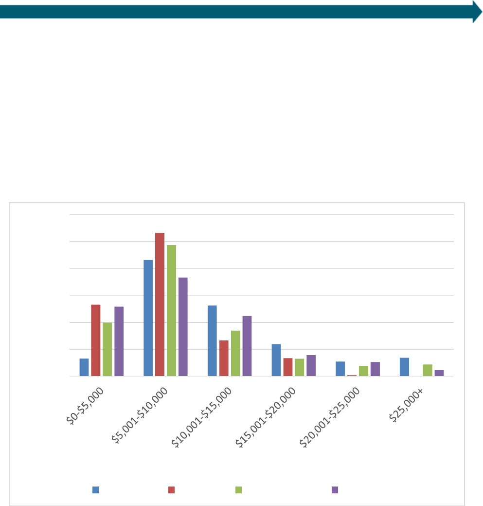
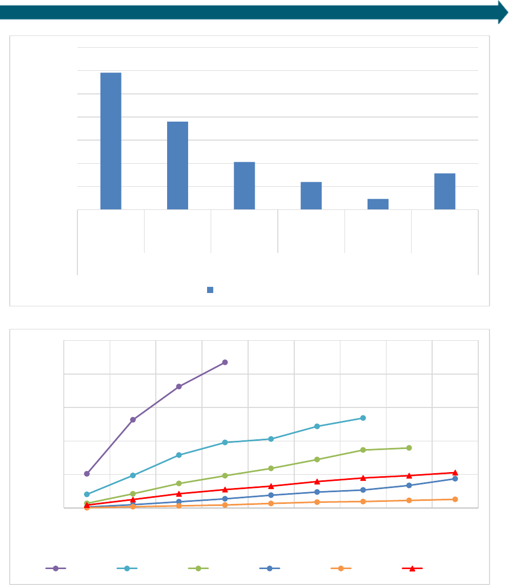
Figure 2 summarizes the principal amounts of loans issued by each program. The amounts participants are
borrowing through these portfolios is concentrated in the $5,000 to $10,000 range (see averages and medians in
Table 3).
Figure 2: Participation by principal amount bin
0%
10%
20%
30%
40%
50%
60%
% of loans
Principal amount bin
CT Smart-E Keystone Michigan Saves NYSERDA
March 2022 www.seeaction.energy.gov 5
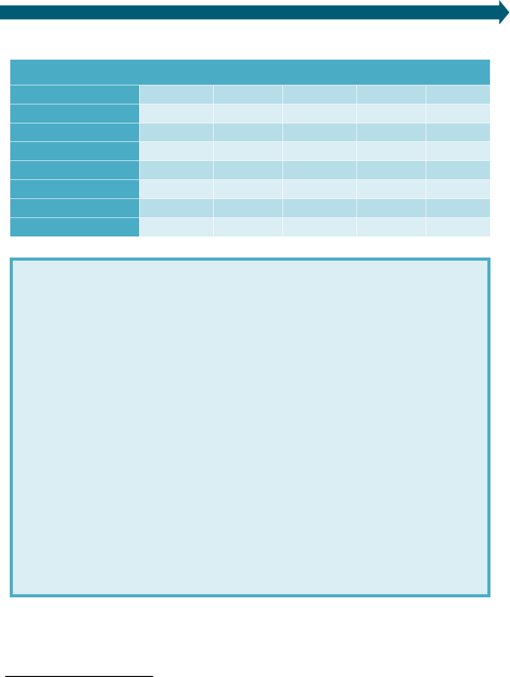
Table 3. Average and median principal amounts, monthly payments, terms, and interest rates
Maintaining loan program data to facilitate performance analysis
To expand the public evidence base on the performance of energy efficiency loans, Berkeley Lab approached a
number of energy efficiency loan programs for this analysis. The four programs that shared data were very
cooperative, and several other programs were willing but ultimately unable to share.
3
A common issue that makes data access challenging is that all the necessary loan data are often not maintained
by a single entity. It is common for different entities to perform different functions – e.g., project approval, loan
origination/underwriting, loan servicing. In some cases, the data on each function reside in different systems.
While there is generally some common identifier (such as a loan ID) that could be used to associate the data, the
level of effort to do so can be significant. By proactively integrating these systems where possible to maintain
consolidated data for analysis, program administrators can help educate and motivate capital providers and lower
the cost of capital for these programs in the future.
Moreover, some programs – including Michigan Saves, Smart-E, and many others – partner with local lenders
(most often credit unions and banks) that make their own loans and maintain their own data. Michigan Saves and
the Connecticut Green Bank demonstrate that some programs gather and consolidate data from multiple lenders
to enable analysis. Where possible, other programs that use many local lenders can help facilitate additional
analysis by gathering their loan data in one central system.
Finally, most if not all programs do not maintain their data in a manner that easily enables time series analysis.
This report studies delinquency and charge-off rates at one moment in time for each program. Programs that can
assemble and maintain a monthly time series of loan status could support more detailed and powerful statistical
analysis.
Berkeley Lab’s report Energy Efficiency Finance Programs: Use-case Analysis to Define Data Needs and
Guidelines provides recommendations on maintaining data to facilitate loan performance analysis; see SEE
Action Network (2014a).
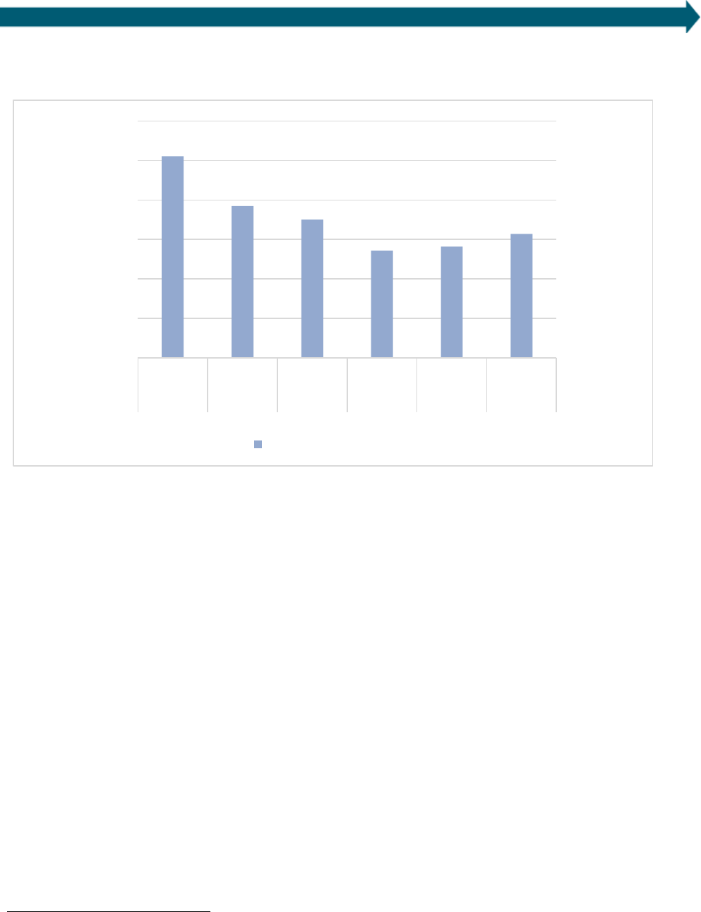
Monthly payments demonstrate the ongoing cash flow burden that a loan presents for participants. Figure 3
presents monthly loan payments for each program. Across the portfolios included in the study, monthly payments
mostly fall into the $51 to $100 per month range. The distribution of monthly payment sizes between Michigan
Saves and Keystone varies little. Compared to the other portfolios, the NYSERDA portfolio has a higher share of
3
The four programs analyzed are among the largest and oldest in the U.S. There are dozens of other energy efficiency financing programs in the
U.S., but few programs offer the high-volume, long-term data (and were willing to share their data), that the four programs provided.
Smart-E
Keystone
Michigan
Saves
NYSERDA
All
programs
Average principal amount
$12,239
$7,594
$9,679
$9,366
$9,137
Median principal amount
$10,094
$7,000
$7,801
$7,971
$7,661
Average monthly payment
$160
$90
$101
$76
$93
Median monthly payment
$139
$80
$85
$65
$80
Average term (months)
92
93
100
166
121
Median term (months)
84
120
120
180
120
Average interest rate
3.5%
6.7%
5.1%
3.8%
5.0%
Median interest rate
4.5%
7.0%
5.0%
3.5%
5.0%
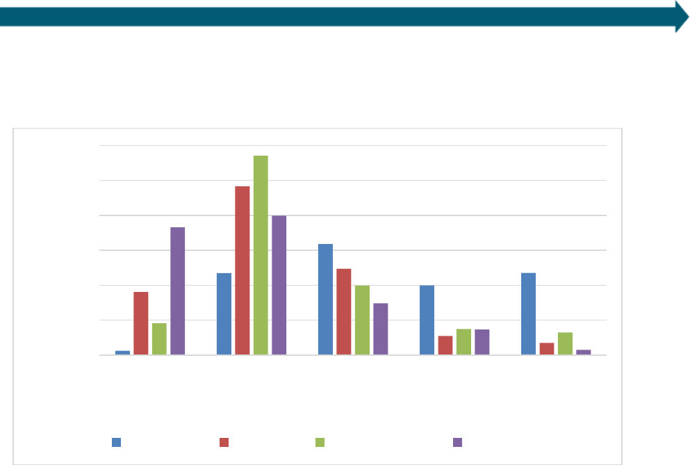
March 2022 www.seeaction.energy.gov 6
loans with monthly payments under $50 per month (37%). The CT Smart-E portfolio has a higher share of loans
with monthly payments above $150 per month (44%). Smart-E principal amounts and area median incomes are
also higher than other programs, suggesting that (1) Connecticut is likely the highest-cost market and (2)
Connecticut borrowers may qualify for larger loans due to their incomes.
F
igure 3. Participation by monthly payment amount
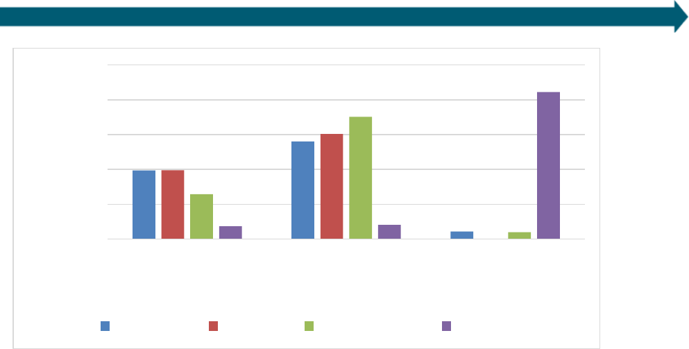
Lo
an term (or tenor) refers to the amount of time until a loan matures. Longer term loans are riskier for lenders
but result in lower monthly payments for borrowers because the repayment is spread over a longer period.
Programs generally offer a limited number of terms (e.g., five years, seven years) and the terms offered may
change over time. Program administrators provided terms for each loan. Loan terms for Keystone, Michigan Saves,
and CT Smart-E are almost entirely ten years (120 months) or less, with terms for over half of loans in each of
those portfolios falling between 61 and 120 months. NYSERDA is the outlier: 84% of their loan terms are 15 years
(180 months), which explains the relatively small monthly payments for NYSERDA loans in Figure 3. The median
loan term across all four portfolios is ten years (120 months) (see Table 3).
0%
10%
20%
30%
40%
50%
60%
<$50 $51-$100 $101-$150 $151-$200 >$200
% of loans
Monthly payment bins
CT Smart-E Keystone Michigan Saves NYSERDA
March 2022 www.seeaction.energy.gov 7
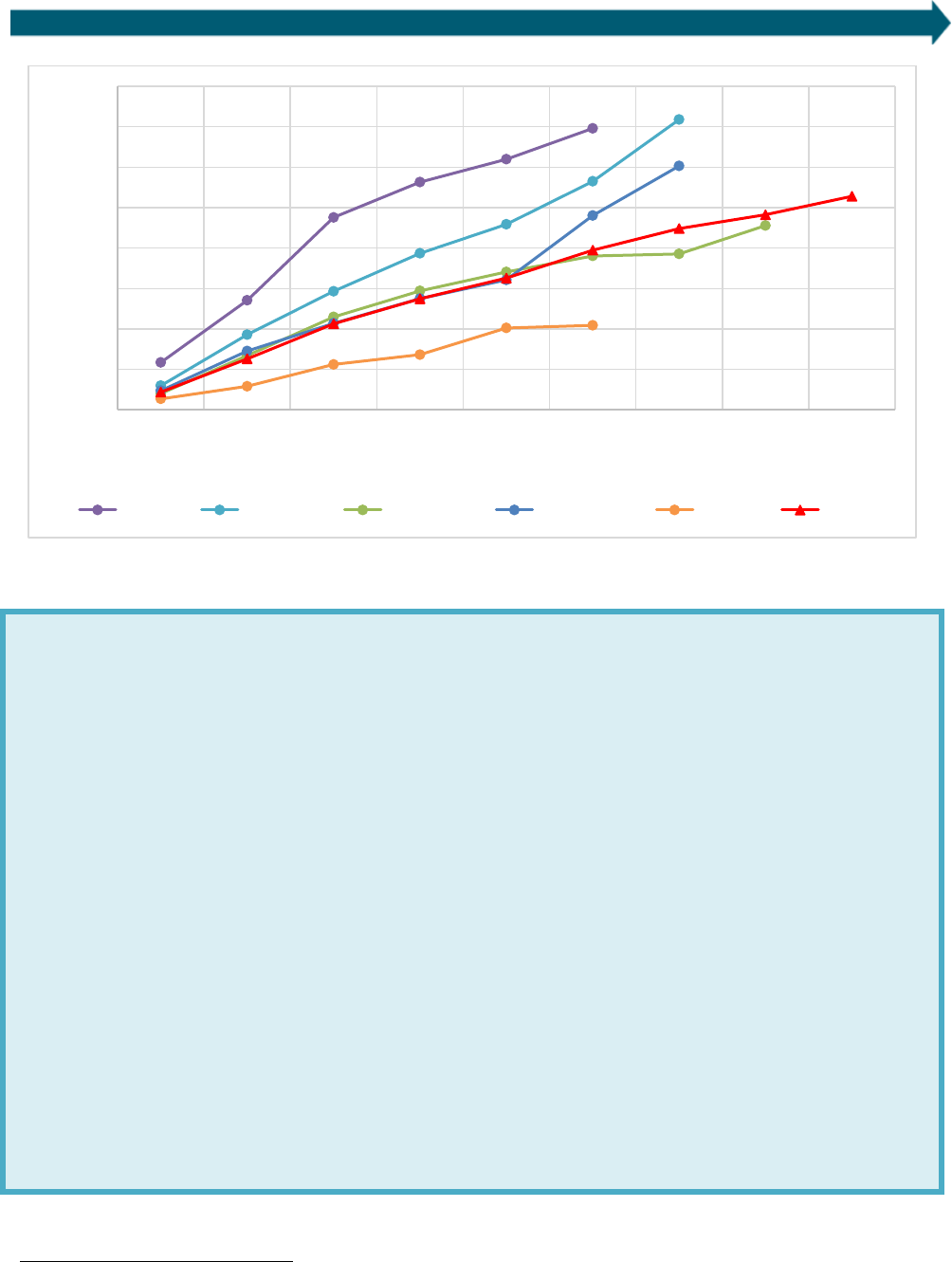
F
igure 4. Share of portfolio participants with different loan terms
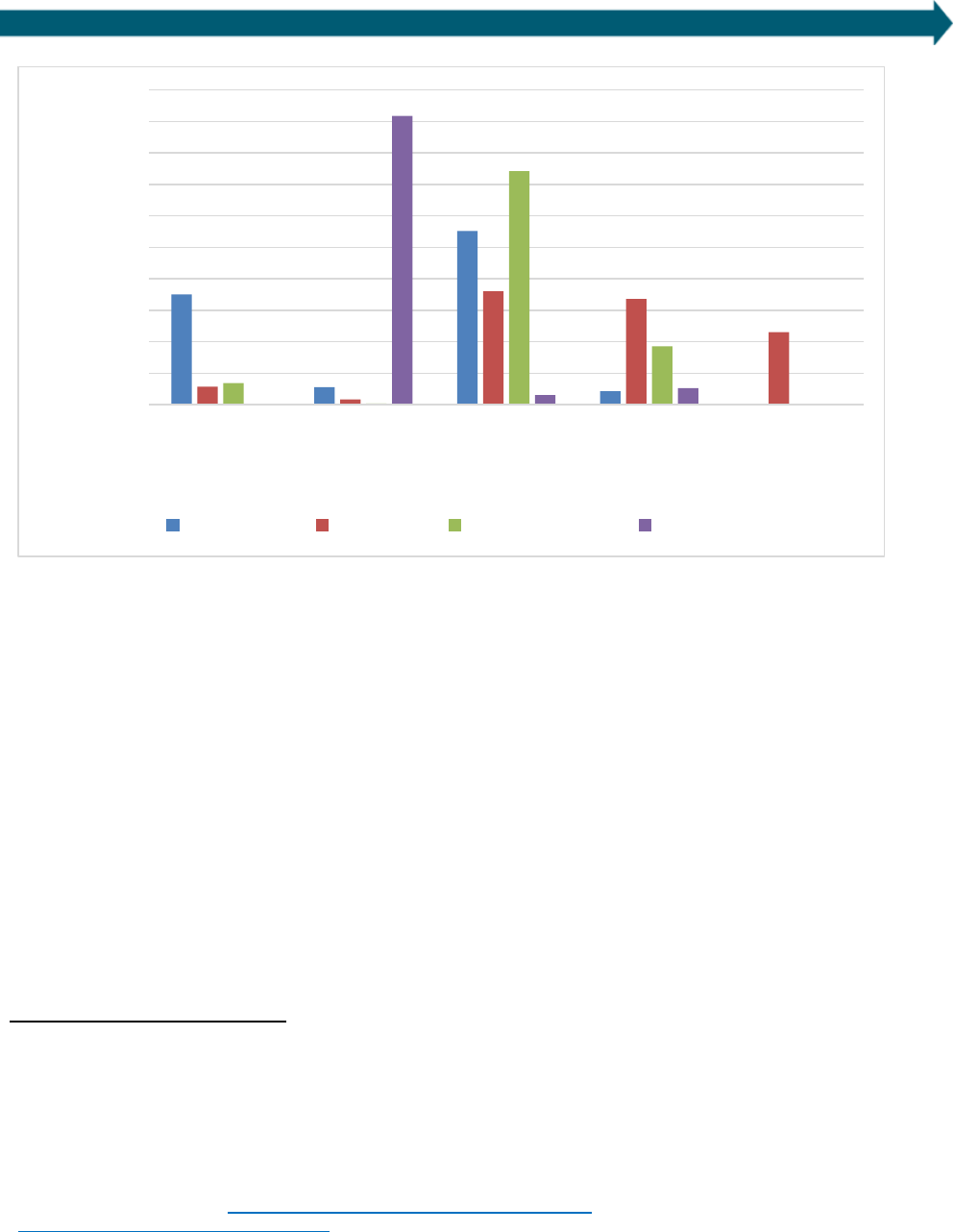
Another factor that impacts payment amounts is the interest rate charged on a loan. Interest rates vary within and
across the four programs. Rates ranged from a low of 0% to a high of 8.99%. Most fall between 4% and 6% with
most NYSERDA loans at 3.49% or 3.99% (see Figure 5). Several factors explain the differences in interest rates
across programs:
• Credit enhancements: Programs that benefit from more generous credit enhancements (such as larger
loan loss reserves) can charge lower interest rates.
• Lender requirements: Different lenders require different returns to participate in these programs. “Pure
”
pr
ivate capital providers generally require higher returns than mission-driven lenders, and programs that
lend public or utility customer dollars have more freedom to set their own rates.
• Timing: Prevailing market interest rates have been low since the Great Recession, but were at times much
higher in the past; this in part explains the higher interest rates charged by Keystone HELP.
• Promotional rates: The Smart-E program offered very low interest rates for a period of time to attract
interest in the program, which explains the large share of Smart-E loans in the first bin.
0%
20%
40%
60%
80%
100%
0-60 61-120 121-180
% of loans
Term bin (months)
CT Smart-E Keystone Michigan Saves NYSERDA
March 2022 www.seeaction.energy.gov 8
F
igure 5. Participation by interest rate
2.2.2. Borrower characteristics
Participant income could impact repayment performance since households with more income have more financial
resources available to make loan payments. Each program collected participant income data differently. Keystone
HELP did not have participant income data (and this portfolio is therefore not included in any analyses that use
income data). NYSERDA reported a debt-to-income-ratio, but not a household-level income metric. The
Connecticut Smart-E Loan program reported a ratio of the median income of a household’s census tract to the area
median income (AMI). Only Michigan Saves reported actual household income. However, every program except
Keystone HELP reported the census tract in which each borrower lives. Berkeley Lab therefore was able to
calculate a common metric – the ratio of median census tract income to AMI – for all programs except Keystone
HELP (see Table 4).
4
Note that this metric describes the income of the census tract in which the home resides but
is not a household-level value.
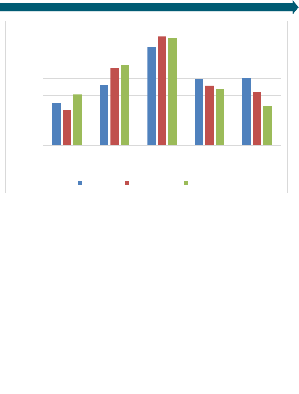
Overall, about two-thirds of participants in these programs are from census tracts where incomes are 80% of the
AMI or higher. The greatest share of participants falls into the 80%-100% AMI bin (see Figure 6). The three
portfolios have a similar distribution across the AMI bins. Overall, across programs the majority of borrowers are
from census tracts with median incomes less than the median income of their statistical area.
5
Relatively few
4
To assess the impact of income across programs in a consistent fashion, Berkeley Lab calculates census tract AMI bands for each program.
This metric is the ratio of census tract-level median household income estimates from the American Community Survey (ACS) to area median
income as defined by the Department of Housing and Urban Development (HUD). This method is consistent with Smart-E’s in the use of census-
tract level median household incomes, but differs in the source of the area median income. Smart-E used ACS Metropolitan and Micropolitan
Statistical Areas, which provided full geographic coverage for Connecticut. New York and Michigan, however, have tracts that are outside these
two types of statistical areas. The HUD area median incomes address this gap and provide county-level incomes alongside statistical area data
incomes. This analysis matches HUD and ACS vintages to the year of loan issuance to account for changes in tract and area incomes over time.
ACS income data can be found at https://www.census.gov/programs-surveys/acs/data.html. HUD income data can be found at
https://www.huduser.gov/portal/datasets/il.html. In this analysis, HUD and ACS incomes are aligned by data release year. HUD data draw on
three-year old ACS estimates for each data release (e.g., 2018 HUD data is based on 2015 ACS data). Given that the ACS incomes cover five
years (e.g., 2014-2018 for the 2018 release), they still overlap with the window of HUD incomes.
5
To see participant incomes by AMI broken into income bins used for the purposes of the Community Reinvestment Act, see Appendix B.
0%
10%
20%
30%
40%
50%
60%
70%
80%
90%
100%
0%-2% 2.01%-4% 4.01%-6% 6.01%-8% 8.01%-10%
% of loans
Interest rate bin
CT Smart-E Keystone Michigan Saves NYSERDA
March 2022 www.seeaction.energy.gov 9
borrowers (10-15%) in each program live in census tracts with median incomes below 60% of area median;
between 30 and 40% of borrowers in each program live in census tracts with median incomes below 80% of area
median.
6
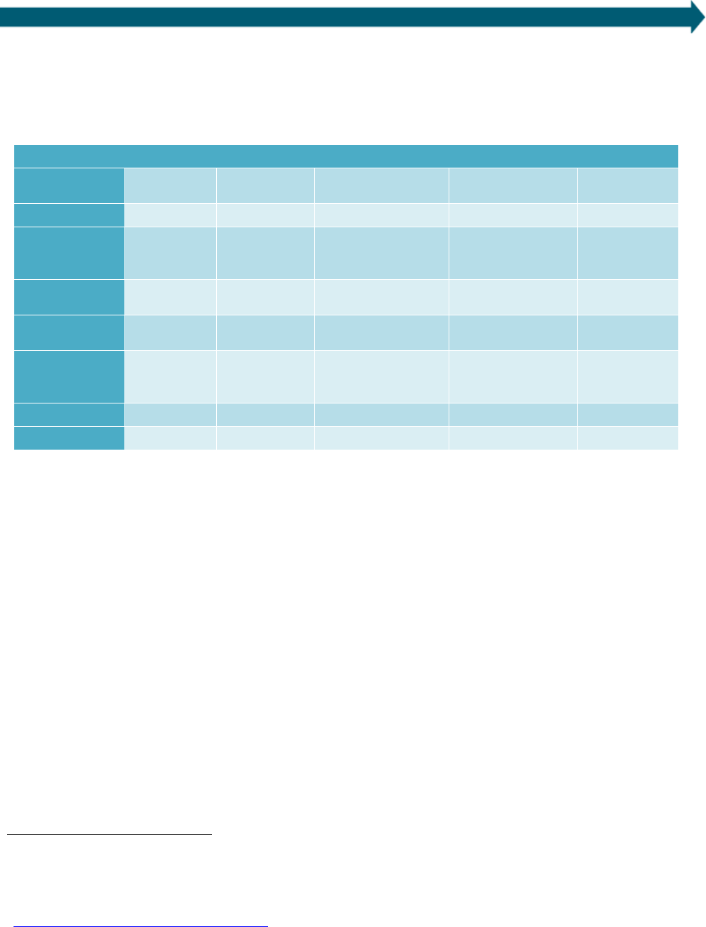
Table 4. Average and median borrower characteristics. (Keystone HELP did not have sufficient data to determine
income metrics.)
Smart-E Keystone Michigan Saves NYSERDA All programs
Median tract
income
$89,858
$63,425
$68,593
$67,152
Median AMI
$95,260
$72,842
$75,736
$74,507
Median tract
income /
median AMI
92.6%
88.8%
85.3%
87.5%
Average tract
income
$93,210
$67,478
$77,529
$74,134
Average AMI
$98,042
$72,637
$87,404
$81,262
Average tract
income /
average AMI
95.2%
93.0%
87.3%
90.8%
Average FICO
739
751
741
729
734
Median FICO
741
754
744
740
745
6
Definitions of low-income households and areas vary, so there is no single way to characterize the share of borrowers in these programs that
are low- and moderate-income (LMI). In the energy sphere, the Low-Income Home Energy Assistance Program uses a household-level eligibility
criterion of 60% of state median income, and the Weatherization Assistance Program also relies on this criterion in some states. 10-15% of
households in the data meet this definition per area (as opposed to state) median income. HUD considers households with incomes less than
80% AMI to be low income and those less than 50% to be very low income for rental housing assistance programs and the HOME program (see
https://www.hud.gov/topics/rental_assistance/phprog
and https://www.huduser.gov/portal/datasets/home-datasets/files/2021-HOME-
IncomeLmts-Memo.pdf). The Community Redevelopment Act (CRA) designates less than 80% AMI as moderate income and less than 50% as
low income. Per Appendix B, 5-8% of borrowers in each program live in census tracts considered low income by the CRA or very low income by
HUD, while about 30-40% would be considered either low- or moderate-income by CRA and low income by HUD.
March 2022 www.seeaction.energy.gov 10
F
igure 6. Participant incomes (by AMI bin) for three portfolios
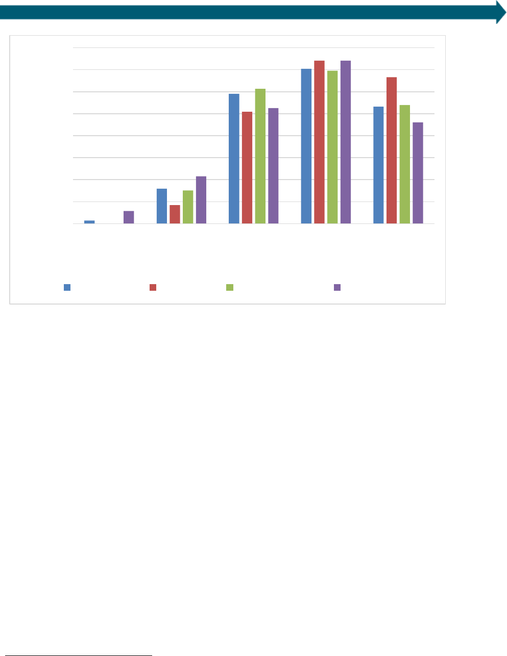
A credit score is a number designed to measure a consumer’s creditworthiness, i.e., it is used to predict the
likelihood that a borrower will fully repay their loan. The most commonly used credit score is the Fair Isaac
Corporation (or FICO) score which ranges from 300 to 850, higher numbers suggesting the borrower is more
creditworthy (see Figure 7 for more).
7
Across the four portfolios, most credit scores are high: the average credit
score is 734 with a median credit score of 745. Importantly, these programs are only available to homeowners,
who as a customer segment have higher credit scores than renters (Li 2016). These scores suggest that the
likelihood that borrowers participating in these programs repay their loans in full is high.
7
Although Berkeley Lab believes that most of the reported scores are FICO scores, Michigan Saves identified one lender that reported Vantage
Scores instead. It is possible that other lenders did so as well.
0%
5%
10%
15%
20%
25%
30%
35%
<60% 60%-80% 80%-100% 100%-120% >120%
% of loans
AMI bins
CT Smart-E Michigan Saves NYSERDA
March 2022 www.seeaction.energy.gov 11
F
igure 7. Participation in four efficiency financing programs by credit score bin
3. Performance analysis
3.1. Methodology
To analyze the data from all portfolios, each loan is assigned a status as either paid-off, delinquent, charged off, or
current.
The definition of charge-offs can vary across loan providers, depending on how they decide when to declare a loan
as a loss.
8
Such determinations may be made if the loan becomes seriously delinquent, but also for other reasons
(e.g., bankruptcy, death of a borrower, etc.). Many lenders automatically declare a loan as charged off if it reaches
a certain delinquency status, often 120 days. This study considers a loan charged off if either (a) the program
identified a loan as charged off or (b) the loan was 120 days or more delinquent. This definition of charge-off is
consistent with those used by comparator products later in this study (auto loans and consumer loans – see
Section 4), to the extent that they specify clear definitions.
Loan providers generally report delinquencies in bins that denote the number of days that have passed without
payment since a payment due date (e.g., 30, 60, 90, 120 days). Since the definition of charge-off covers loans 120
days or more delinquent, delinquent loans are those that have not been paid 30-120 days after the payment due
date.
Customers may pay their loans off at or before the original maturity date. A loan is paid-in-full if a program
identifies it as such or the remaining balance is zero.
8
When a lender declares a loan to be charged off, it declares the loan as a loss on its accounts and often transfers collection responsibilities to a
collection agency. If the collection agency reports to credit bureaus, the loan will now appear as a charge-off on a borrower’s credit report. The
borrower is still obliged to repay the loan.
0%
5%
10%
15%
20%
25%
30%
35%
40%
300-600 601-660 661-720 721-780 781-850
% of loans
Credit score bin
CT Smart-E Keystone Michigan Saves NYSERDA

March 2022 www.seeaction.energy.gov 12
A loan is current if it is neither charged off, delinquent, nor paid-in full. Current loans are actively in repayment but
not in any form of distress.
Delinquency rates presented in this report are the share of active (not charged off and not paid off) loans that are
30-120 days behind on payments. The delinquency rate can be expressed both in terms of the total remaining
balance of loans that are delinquent and the number of delinquent loans.
=
=
For example, if a loan portfolio has $1,000,000 in outstanding principal balance from 1,000 active loans and 60 of
those loans with a total of $50,000 in outstanding principal balance are 30-120 days delinquent, then the portfolio
would have a dollar-based delinquency rate of 5% ($50,000/$1,000,000) and count-based delinquency rate of 6%
(60/1,000).
The cumulative gross loss rate
9
is the total dollars charged off after some number of years for loans originated at
least that long ago (but not past their term) as a share of the original balance of those loans. The cumulative gross
loss rate can be calculated for each year of seasoning (i.e., how much time has passed since the program issued
the loan). Loans that have seasoned for five years, then, are part of the loss rate for years one through five but not
for years after five.
=
In the hypothetical portfolio with $1,000,000 in outstanding principal balance from 1,000 loans, assume that the
original loan pool was 1,050 loans (i.e. 50 have already charged off). If the original principal balance of those 1,050
loans was $2,000,000 and the 50 which were charged off totaled $40,000, then the cumulative gross loss rate
would be 2% ($40,000/$2,000,000).
Regression analyses determine the drivers of delinquency and charge-off and unpack differences in performance
across the portfolios (see Section 3.2.3 for details).
3.2. Findings
3.2.1. Delinquency and loss analysis
Figure 8 presents 30-120-day delinquency rates for each program. The sample sizes in this figure differ from those
in Figure 10 because the delinquency rate calculation only considers current loans and excludes any paid-off or
charged-off loans. Overall, the 30-120-day delinquency rate for loans in the four portfolios is 1.57%.
NYSERDA delinquency rates for the On-Bill Recovery Loan – an on-bill loan – are much higher than those for its
Smart Energy Loan product, explaining its high overall delinquency rate. Due to the structure of the program, any
delinquency on a utility bill also results in a delinquency on the on-bill loan. When NYSERDA on-bill loans – which
are somewhat atypical – are removed from the pool, the 30-day delinquency rate drops to 1.14% Notably,
NYSERDA on-bill loss rates are not higher than those of the off-bill Smart Energy Loan, indicating that most of these
delinquencies do eventually cure. Section 3.2.3.3 discusses this issue further. As also noted in Section 3.2.3.3, the
difference in delinquency rate between Smart-E loans and the lower-delinquency programs is not statistically
significant (Smart-E has the smallest loan count of the programs in this study).
9
As discussed in Section 4, most loan performance indices look at net losses, e.g., losses minus recoveries (any monies recovered after a loan is
charged off). Because no recovery data was available for these portfolios, this analysis reports gross losses instead of net losses.
March 2022 www.seeaction.energy.gov 13
F
igure 8. 30-120-day delinquency rates by program
To understand how losses depend on loan seasoning, Figure 9 presents cumulative gross loss rate over time for
each program with respect to years of loan seasoning. Each data point in this figure shows the cumulative gross
loss rate since initial loan closing. Since the loss rates are cumulative, they increase over time for all four portfolios.
The loss rates are sensitive to both vintage effects and small loan pools. The number of loans that have seasoned
eight years, for example, is much smaller than the number that has seasoned two. This figure addresses this issue
by excluding loan vintages with total principal amounts under $5M, which is why some curves do not extend as far
as others. Vintage effects, such as higher loss rates for loans issued before the 2008 financial crisis could affect
Keystone loans in particular.
0.0%
0.5%
1.0%
1.5%
2.0%
2.5%
3.0%
n=5485 n=10827 n=2782 n=14145 n=33239
Keystone Michigan Saves Smart-E NYSERDA Overall
Share of Outstanding Balance
Delinquency Rate (Dollars)
March 2022 www.seeaction.energy.gov 14
F
igure 9. Cumulative gross loss rates by program and years of seasoning
Close examination of Figure 9 shows that more losses occur in the early years after loan issuance than in later
years. For example, looking at the overall cumulative loss curve, losses in year 8 are 5.3%. If the loss rate was
constant over time, losses in years 2, 4, and 6 would be 1.3%, 2.6%, and 4.0% respectively. In fact, those loss rates
are 2.1%, 3.3%, and 4.5%, showing that the loss curve is somewhat concave (bowed downward). This behavior is
visually apparent for all the individual portfolios except Keystone, which again may be affected by vintaging (i.e., a
loan’s issue year) effects of the financial crisis – meaning that loans with a good deal of seasoning (which are the
ones that date to before the crisis) have higher loss rates than if the financial crisis had not occurred. Since a large
share of the more seasoned loans in the pooled portfolios are Keystone loans (consistent with Figure 9), this may
also affect the latter years in the overall curve.
Figures 10 and 11 show the relationship between loan performance and credit score across the pooled portfolios.
Figure 10 shows how delinquency rates decline as credit score increases; Figure 11 demonstrates how cumulative
gross loss rates increase as credit score declines. Loans to customers in the highest credit score bin have one-third
of the delinquencies of the combined portfolios as a whole. Figure 11 shows a similar relationship between
cumulative gross losses and credit score: the higher the credit score, the lower the losses. Differences are apparent
in the first year of seasoning and grow as the loans mature. After three years of seasoning, loans issued to
customers with the lowest credit scores (300-600) have cumulative gross loss rates more than 21 percentage
points higher than customers with the highest credit scores (781-850). For loans issued to customers in the two
highest credit score bins, cumulative gross losses are less than 5% after eight years.
0%
1%
2%
3%
4%
5%
6%
7%
8%
0 1 2 3 4 5 6 7 8
Cumulative Gross Loss Rate
Years Seasoned
Smart-E Keystone Michigan Saves NYSERDA Overall
March 2022 www.seeaction.energy.gov 15
F
igure 10. Delinquency (share of outstanding loans) by credit score bin
F
igure 11. Cumulative gross loss by credit score bin
Loan performance does not show the same degree of sensitivity to census tract income, as shown by AMI bands in
Figures 12 and 13. Delinquency and loss rates decline as income increases, but not to as great an extent as they do
with credit score increases. For example, delinquency rates in the lowest credit score bin (300-600, Figure 10) are
about 12 times higher than the delinquency rates in the highest credit score bin (781-850), but delinquency rates
in the lowest AMI band (0-60%, Figure 12) are only 1.9 times as high as in the highest AMI band (>120%). As shown
0%
1%
2%
3%
4%
5%
6%
7%
n=388 n=2698 n=9365 n=11839 n=8047 n=33239
300-600 601-660 661-720 721-780 781-850 Overall
FICO Bin
Share of Outstanding Balance
(Delinquency)
Delinquency Rate
0%
5%
10%
15%
20%
25%
0 1 2 3 4 5 6 7 8
Cumulative Gross Loss Rate
Years Seasoned
300-600 601-660 661-720 721-780 781-850 Overall
March 2022 www.seeaction.energy.gov 16
in Figure 13, cumulative gross loss rates are highest in the lowest AMI band (0-60%) but are only higher than the
loss rate in the highest AMI band by five percentage points after five years.
10
Figure 12. Delinquency (share of outstanding loans) by program and AMI band
10
The cumulative gross losses by income band do not include loans from Keystone due to the lack of census tract data in that dataset. Since
Keystone has some of the oldest loans in the dataset, its absence in this figure contributes to the loss rates not extending to year eight as they
do for most credit score bins in Figure 11.
0.0%
0.5%
1.0%
1.5%
2.0%
2.5%
3.0%
n=3355 n=5908 n=7847 n=4199 n=3499 n=33239
0-60% 60%-80% 80%-100% 100%-120% >120% Overall
Share of Oustanding Loans
(Delinquency Rate)
AMI Band
Delinquency Rate (Dollars)
March 2022 www.seeaction.energy.gov 17
Figure 13. Cumulative gross loss rates by AMI band
The relationship between income and credit, and implications for programmatic lending
It is commonly believed that high-income households also have high credit scores. In fact, there is generally a small
positive correlation between income and credit score, but this correlation is lower than might be expected. In the pooled
data, the correlation
11
between the median household income of the census tract where borrowers live and their credit
scores is only 0.11 – meaning that census tract median income explains only about 11% of the variation in credit scores
and vice versa. Moreover, this low correlation does not appear to be due to use of a census tract-based income. In
Michigan, the correlation between census tract median income and credit score is similar at 0.10; the correlation
between household income and credit score is considerably lower, at 0.015.
These findings do not suggest that income per se is not important to understanding loan performance. All the programs
in this analysis generally include a debt-to-income threshold in their loan underwriting. (The partial exception is
NYSERDA, which allows higher than traditional DTI ratios with satisfactory mortgage payment history under its “Tier
2” underwriting option, and in January 1, 2019 eliminated maximum DTI ratios for applicants with FICO scores greater
than 780). Rather, the findings suggest that, for households that pass the debt-to-income screens implemented by the
programs (see Table 2), income matters relatively little – and less than credit – for understanding delinquencies and
losses. These DTI ratios may screen out many low-income households; this analysis does not explore whether
alternative DTI thresholds could be set.
This report finds that credit score predicts delinquencies and charge-offs far better than income. Figures 10 through 13
demonstrate this finding in the raw data, and the regression analysis in Section 3.2.3 confirms that the association
between performance and credit is much stronger than that between performance and income. These findings suggest
that lenders can expect strong payment performance from households in lower-income areas that (1) have strong credit
and (2) meet debt-to-income screens similar to those in these programs. Many households in the data fit this description.
Of participating households in census tracts below 100% AMI, 48% had credit scores above 740 – similar to the share of
participating households in census tracts above 100% AMI with credit scores above 740 (56%).
11
“Correlation” refers to Pearson’s correlation coefficient.
0%
1%
2%
3%
4%
5%
6%
7%
8%
0 1 2 3 4 5 6 7 8
Cumulative Gross Loss Rate
Years Seasoned
0-60% AMI 60%-80% AMI 80%-100% AMI 100%-120% AMI >120% AMI Overall

March 2022 www.seeaction.energy.gov 18
3.2.2. Prepayment
This section briefly discusses prepayment rates in the studied portfolios. Prepayment occurs when a borrower pays
the loan in full prior to the scheduled loan maturity.
12
All values in this section exclude Smart-E loans, since Smart-
E program data did not include the date loans were prepaid.
Most loans in the studied portfolios are still active. Among loans that have come to term (loans whose scheduled
maturity was prior to the end date of each portfolio’s dataset), borrowers reach about 70% of the loan term on
average before paying in full. This average combines loans prepaid at various points in the term with loans carried
to the full term. It should be noted that the average term of these loans is 56 months; most of these loans are
Keystone loans with five-year terms. These loans are not representative of the larger pool of loans since very few
longer-term loans or loans from other programs have come to term.
The cumulative prepayment rate is the share of the original loan balance that has been prepaid after a period of
time. For example, the cumulative prepayment rate for loans that have seasoned for at least three years is the
value of loans that has been fully prepaid through those three years as a share of original balance for those loans.
In the pooled loans, after three years, about 17% of the original loan balance has been fully prepaid. After six
years, that cumulative prepayment rate is about 32%. The data do not provide enough information for us to
include partial prepayments in these calculations, so the figures above are underestimates of the true prepayment
rate in these portfolios.
3.2.3. Regression analysis
This regression analysis builds on the high-level program, credit, and income trends in the previous section by
parsing the impact of the various determinants of loan performance discussed above. The logistic regression
measures the change in the likelihood of delinquency and charge-off depending on borrower and loan
characteristics: principal amount, income bin, credit score, loan seasoning, interest rate, and which program issued
the loan. The regression demonstrates the impact of each factor while holding all the others constant. See
Appendix A for more details on the regressions.
Our analysis splits out two subprograms in NYSERDA, On-Bill Recovery and Smart Energy, to account for
differences in program design and customer characteristics in these programs. Note that the regression models
presented here include income as a variable, and therefore exclude Keystone HELP due to lack of income data.
When removing income and adding Keystone HELP back to the analysis, results for the other variables are similar
to those presented here. For regression tables, see Appendix A.
3.2.3.1 Credit score regression results
Credit score stands out as a consistent, statistically significant predictor of delinquency and charge-off. Higher
credit scores are associated with lower chances of delinquency and charge-off for every portfolio. Considering
Figure 10, this is not a surprise.
The association between credit score and charge-off is larger than the association between credit score and
delinquency (see Table A-1). For charge-offs, a 100 point increase in credit score is associated with a 5.81
percentage point decrease in the chances a loan is charged off.
13
A 100-point increase in credit score is associated
with only a 1.06-percentage point reduction in the chance of delinquency. Still, both relationships have strong
statistical significance.
14
Program-specific regressions show similar impacts; while the magnitude of the
12
Lenders generally prefer for loans to be carried to term. If a loan is prepaid, then the investor will not receive part of the interest payments
that they may have been expecting.
13
The term ‘percentage point’ is used to distinguish a difference in percentages from a “percent of a percent” change; “percentage points”
refers to the former. For example, a change from 1% to 2% is a change of one percentage point.
14
Note that the positive correlation between borrower credit score and loan performance is not unique to energy efficiency loans.

March 2022 www.seeaction.energy.gov 19
relationships varies somewhat, in all cases higher credit scores are associated with lower chances of delinquency
and charge-off, and in all cases the relationships are statistically significant at conventional levels of significance.
3.2.3.2 Income regression results
Across all portfolios combined, relative to loans in the 0-60% AMI band, the chance of charge-off decreases for
loans in the three highest income bands (80-100% AMI, 100-120% AMI, > 120% AMI). These differences are
statistically significant. Holding all else equal, households in the > 120% AMI band have a charge-off rate 1.98
percentage points lower than those in the < 60% AMI band. When examining delinquency, loans in the two highest
income bands (100-120% AMI, > 120% AMI) show statistically significantly lower rates of delinquency than loans in
the lowest income band. Both the high-income bins show a rate lower by 0.50 percentage points relative to the
rate in the <60% AMI band (see Table A-2).
In single-portfolio regressions, the impacts of income on charge-off were often, but not always, statistically
significant. The impact of income on delinquency were almost never statistically significant. This difference
between pooled and single-portfolio results suggests that the scale of the study – in these regressions (which do
not include Keystone HELP), about 25,000 loans – is important to demonstrate a relationship between income and
loan performance, especially in the case of delinquency. When pooling the programs, the relationships emerge;
however, single portfolios do not have adequate sample size to clearly demonstrate them. This stands in contrast
to credit score, where associations with both delinquency and charge-off are clear and large even in single-
portfolio regressions.
One possible explanation for the relatively weak relationship between income and loan performance (also shown
in Figure 12) is that the income variable is based on the median income of the census tract, rather than the income
of the household itself. Census tract income is a blunt signal of actual household-level income. However, the data
do not suggest that use of census tract incomes, rather than household incomes, is consequential for these results.
For Michigan Saves – the one program with available household-level income data – the correlation between
household income and census tract median income is relatively weak (0.20). However, the relationships between
household income and charge-off/delinquency are not clearly different than those using census tract median
incomes. Regression analysis on the Michigan Saves data shows that household incomes – like census tract median
incomes – are associated with charge-offs, with a $10,000 increase in income decreasing the chance of charge-off
by 0.26 percentage points. Household income is not a statistically significant predictor of delinquency in the
Michigan Saves data. Both results are similar to the results of regression analysis on the Michigan Saves program
using census tract incomes.
3.2.3.3 Program regression results
The regression analysis generally confirms the differences in overall program delinquency and loss rates presented
in Section 3.2.1. Connecticut Smart-E has the lowest charge-off rates when controlling for the other factors
discussed in this section, and NYSERDA’s Smart Energy loans have the highest.
15
Smart-E and both NYSERDA
programs have the highest delinquency rates, while Keystone and Michigan Saves have the lowest. It is beyond the
scope of this study to consider program-specific features that might explain these differences in performance.
Overall, while some of these differences are statistically significant, they are relatively small in magnitude.
3.2.3.4 Other regression results
In addition to credit score and income, the regression analysis also estimates the impact of principal amount,
interest rate, and seasoning on loan performance. This section reviews only the results for regressions on the
combined portfolios.
15
This study observes higher chances of delinquency in NYSERDA’s on-bill loans relative to its Smart Energy loans, consistent with the findings
in Deason (2015) several years earlier in the program’s lifespan. However, Deason (2015) did not study charge-offs. The results in this report
show that NYSERDA’s on-bill loans are not charged off more often than its Smart Energy loans; in fact, controlling for other factors, they are
charged off less often, though the difference is not statistically significant.

March 2022 www.seeaction.energy.gov 20
Principal amounts have a statistically significant association with charge-offs, but not with delinquencies. Even for
charge-off, the effect is relatively small: a $10,000 increase in principal amount only increases the chance of
charge-off by 0.46 percentage points.
A 1-percentage point increase in interest rate increases the chance of charge-off by 2.29 percentage points for all
programs combined. Interest rate does not have a statistically significant impact on delinquency.
Loan seasoning does have clear associations with loan performance. A loan’s chance of charge-off increases by
0.76 percentage points for each year it has seasoned, while the chance of delinquency decreases by 0.11
percentage points for each year of seasoning. Seasoning can only increase the chances a loan becomes charged
off, since charge-off can occur only once. On the other hand, loans can and do go in and out of delinquency. The
fact that the relationship is reversed for delinquency suggests that borrowers who have trouble repaying their
loans tend to get in trouble relatively quickly – which is consistent with the shape of the loss curves in Figures 9,
11, and 13.
4. Comparators
A key purpose of this research is to help assess whether energy efficiency loans perform differently than other
comparable financial products. Observers have long theorized that energy efficiency loans may carry a
performance premium. If so, there may be a number of potential reasons:
• These loans generate their own cash flow (through energy cost savings) to help service the debt.
• Participating borrowers have particular characteristics that make them likely to repay, whether easily
observable (e.g., credit scores) or not (e.g., adoption of energy efficiency measures may be a sign that a
borrower tends to be frugal or pay close attention to costs, so these products might select for borrowers
with an otherwise unobservable tendency to repay reliably).
• Participants see clean energy improvements as an investment in their home and treat that investment
similar to the way they would a loan that is secured by the home.
• Borrowers may seek these loans out because they believe they are doing something beneficial for the
environment and would see failing to make payments as undermining their good deed.
• Program structures and safeguards (e.g., careful contractor vetting and approval as well as well-executed
project approval and underwriting processes) help forestall predatory lending and otherwise avoid
abusive lending practices that may be present to a greater extent in other loan pools.
To contextualize these results, this section compares the delinquency and charge-off performance of the energy
efficiency loans in this study with several indices of loan performance. These comparisons cannot specifically
determine whether efficiency loans carry a performance premium relative to otherwise similar non-efficiency
loans, but they do help situate their performance relative to better-known asset classes.
4.1. Methodology
The analysis first identifies several relevant comparator financial products. There is no one perfect comparator to
residential energy efficiency loans. In a sense, energy efficiency loans are a specialized type of home improvement
loan; however, most home improvement loans are for more expensive renovation projects and may be secured by
the home. Instead, Berkeley Lab chose general consumer loans and auto loans as comparators.
16
Consumer loans
are broadly similar to energy efficiency loans in that they are generally unsecured loans made to individuals,
although consumer loans are made without regard to dwelling ownership (or rental) status. While different types
of consumer loans (and consumer loans to different customers) vary substantially, in general these loans have
similar principal amounts on shorter terms (and therefore higher monthly payments), and carry considerably
16
While mortgages are another potential comparator, the fact that mortgages are secured by the home, and the much longer loan terms of
many mortgages, make them less suitable for comparison.

March 2022 www.seeaction.energy.gov 21
higher interest rates than the studied energy efficiency loans.
17
Auto loans differ in that they are secured by the
vehicle, meaning that one might expect somewhat stronger repayment performance. Average auto loan amounts
and monthly payments are higher than residential energy efficiency loans and average terms are shorter, while
interest rates are similar for new cars and higher for used cars. Average credit scores for new car loan borrowers
are similar to the energy efficiency loan borrowers, while average credit scores for used car borrowers are
considerably lower.
18
Most importantly, both consumer loans and auto loans have very large markets and are well-
characterized by public loan indices.
Comparator loan performance data comes from three sources:
• Data maintained by the Federal Reserve (“Fed”). The Fed data
19
cover loans reported by brick-and-mortar
banks, including credit card loans as well as non-credit card personal loans.
• Loan performance indices maintained by Kroll Bond Rating Agency (KBRA). The KBRA Marketplace
Consumer Loan indices cover securities comprised of loans made by online lenders (often known as
FinTech loans), separated into three tiers by the average credit quality served by each lender. The analysis
uses data for Tier 1 loans in the KBRA index, which include deals with average credit scores from 710 to
740 (and are therefore the appropriate comparator for energy efficiency loans). KBRA also reports two
auto loan indices, one for prime auto loans and one for non-prime auto loans. While there is no universal
division between the two, non-prime loans are generally loans to borrowers with credit scores in the mid-
600s and below. The analysis therefore focuses on the prime auto loan index.
• Loan data sampled from credit reports by TransUnion. While TransUnion data cover auto loans, bankcard
loans, and unsecured personal loans, the analysis only includes their data on unsecured personal loans
here. TransUnion usefully subdivides these loans further by type of lender (e.g., banks vs. credit unions),
providing greater resolution on personal loans than the other indices.
The comparisons focus on the same two performance metrics used elsewhere in this report: 30-day delinquencies
and cumulative gross losses. All indices define 30-day delinquencies in the same way that this report has defined
them.
In terms of losses, earlier sections of this report show loss curves over time. For most comparators the data to
support these curves are not available, though KBRA helpfully supplied us with the requisite data for two of their
loan indices. Most comparators instead report an annualized loss rate, which indicates the share of the portfolio
that would be expected to be lost in a year. Annualized losses are readily calculated for large portfolios that can be
assumed to be at “steady state,” meaning that loans of many different maturities are present and the overall
seasoning of the portfolio is not changing significantly over time. In the energy efficiency loan data, this is not the
case: the majority of loans are still relatively unseasoned. In this situation a common ratings agency practice is to
“gross up” cumulative losses to the loss rate expected at loan maturity. However, few loans in the portfolios
studied here have reached maturity (nearly none in some portfolios). Instead of attempting to forecast losses at
maturity, the annualization method employed here divides losses at the time they are observed by the average
seasoning of the loans. This method essentially assumes losses occur at a constant rate over time, which is not
consistent with Figure 9; however, there is no ready alternative. Since loss rates do decline somewhat with
seasoning, this method likely overestimates the loss rates in a mature portfolio of these efficiency loans.
Even setting aside this difference in annualization method, this annualized loss calculation differs from the
comparators in two other respects:
17
See the following sources regarding unsecured consumer loans: https://www.lendingtree.com/personal/personal-loans-statistics/;
https://www.fool.com/the-ascent/research/personal-loan-statistics/;
https://fred.stlouisfed.org/series/TERMCBPER24NS; https://www.chamberofcommerce.org/personal-loan-statistics.
18
See https://www.experian.com/content/dam/noindex/na/us/automotive/finance-trends/state-of-auto-finance-q2-2021.pdf for data on auto
loans and auto loan borrowers.
19
See https://www.federalreserve.gov/releases/chargeoff/
March 2022 www.seeaction.energy.gov 22
• Gross rather than net charge-offs. KBRA reports net charge-off rates that include revenues from
recoveries.
20
This analysis could not access data on recoveries from energy efficiency loans, as discussed
above, so the calculated charge-off rates are gross rates. Since gross charge-off rates are an upper limit on
net charge-off rates (only reached if recoveries are zero), these rates may be overestimates of the net
charge-off rates from the programs studied. Thus, this report’s comparisons to net charge-off indices may
underestimate the true relative performance of energy efficiency loans included in this report.
• Berkeley Lab annualizes charge-offs differently. The Fed and KBRA indices draw from a large volume of
loans and calculate loss rates solely within the month or quarter that are reported, then multiply (by 12 or
4, respectively) to extrapolate those losses to annual values. The energy efficiency loan pools are much
smaller, resulting in a good deal of random variance month-to-month and year-to-year. Therefore, as
discussed in Section 3.2.1, the method used here annualizes in the reverse direction: it calculates the net
loss rate of each portfolio across its entire lifetime, and then annualizes that value by dividing by the
average seasoning of each portfolio.
4.2. Findings
The Fed data are reported quarterly, while KBRA indices are calculated monthly. To generate the comparators to
the energy efficiency loan data, Berkeley Lab averages the rates reported by each index in the months/quarters of
each of the four program datasets (see Table 1).
Figure 14. Delinquency rates, energy efficiency loans and comparators
The pooled 30-day delinquency rate across all four energy efficiency loan portfolios is lower than all comparators,
including secured prime auto loans (see Figure 14). The energy efficiency loan delinquency rate is 1.57%, a fair bit
lower than the 2.15% rate of non-credit card consumer loans (from the Fed data), as well as the 1.75% rate for
unsecured personal loans from banks and the 2.6% rate for unsecured loans from credit unions.
Figure 15 presents the equivalent data for charge-offs (gross charge-offs for the energy efficiency loans; net
charge-offs for comparators) for two KBRA indices for which KBRA shared data on losses over time to facilitate this
analysis. The comparator loss rates in this graphic are principal-weighted averages of KBRA’s loss rates by annual
20
Recoveries are money that a lender has been able to recover from a loan that has been charged off, e.g., through a collection agency or sale
of the vehicle in the case of auto loans.
0.0%
0.5%
1.0%
1.5%
2.0%
2.5%
3.0%
3.5%
4.0%
Pooled EE
loans, all
programs
Unsecured
personal
loans from
banks
(TransUnion)
Auto loans,
prime only
(KBRA)
Non-credit
card cons
loans (Fed)
Consumer
loans, Tier 1
(KBRA)
Consumer
loans, with
credit (Fed)
Unsecured
personal
loans from
credit unions
(TransUnion)
FinTech
unsecured
personal
loans
(TransUnion)
Share of Outstanding Loans
(Delinquency Rate)
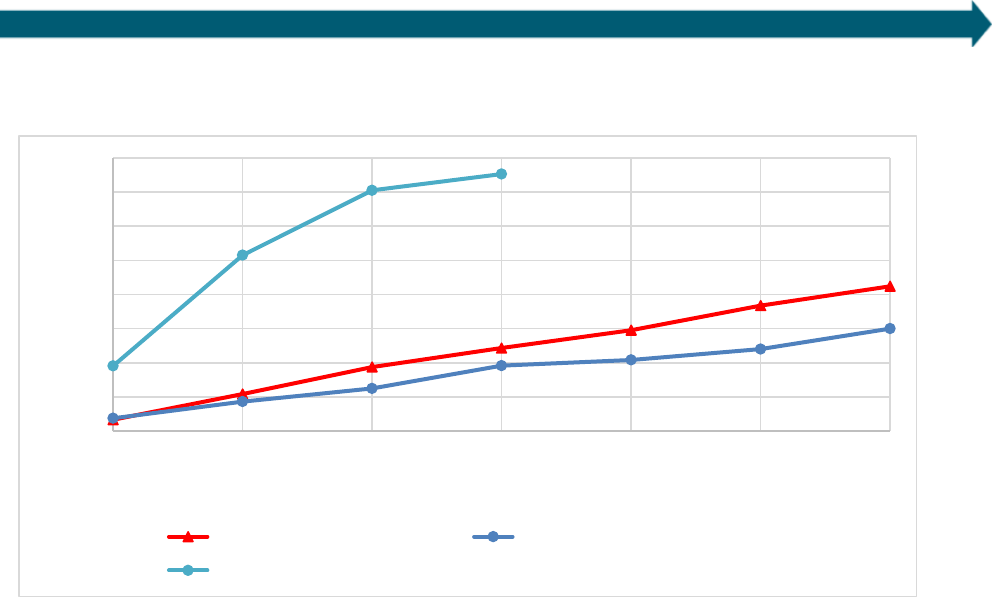
March 2022 www.seeaction.energy.gov 23
loan vintage from 2006-2019, in the case of auto loans, and from 2016-2019 for consumer loans (as the index
began in 2016).
Figure 15. Cumulative loss rates for, energy efficiency loans (gross), KBRA Prime Auto (net), and Tier 1 Consumer
Loans (net)
Losses for energy efficiency loans are comparable to prime auto losses and are much lower than Tier 1 consumer
loan losses
, despite the fact that the energy efficiency loan losses are gross rather than net. After three years of
seasoning, the pooled energy efficiency loans have a cumulative gross loss rate of 2.4%, while the KBRA prime auto
loans and Tier 1 consumer loans have cumulative net loss rates of 1.9% and 7.5% respectively.
Finally, Figure 16 shows a comparison between the annualized loss metric for the energy efficiency loans – again,
an imperfect metric as described above – and annualized loss rates for comparators. In the same manner as the
delinquency comparisons, the comparator loss rates are calculated by averaging the rates reported by each index
in the months/quarters of each of the program datasets. Given this annualization method, one could argue that
comparator rates should in some way average delinquency and loss rates across the portfolios’ lifetimes. In
practice, with the notable exception of the 2008/09 recession (which affected only early loans in the Keystone
program), comparator delinquency and loss rates have been very stable during the period of observation, so the
simple approach suffices.
0%
1%
2%
3%
4%
5%
6%
7%
8%
0 1 2 3 4 5 6
Cumulative Gross Loss Rate
Years Seasoned
Efficiency Portfolios Overall (Gross) KBRA Prime Auto (Net)
KBRA Tier 1 Consumer Loans (Net)
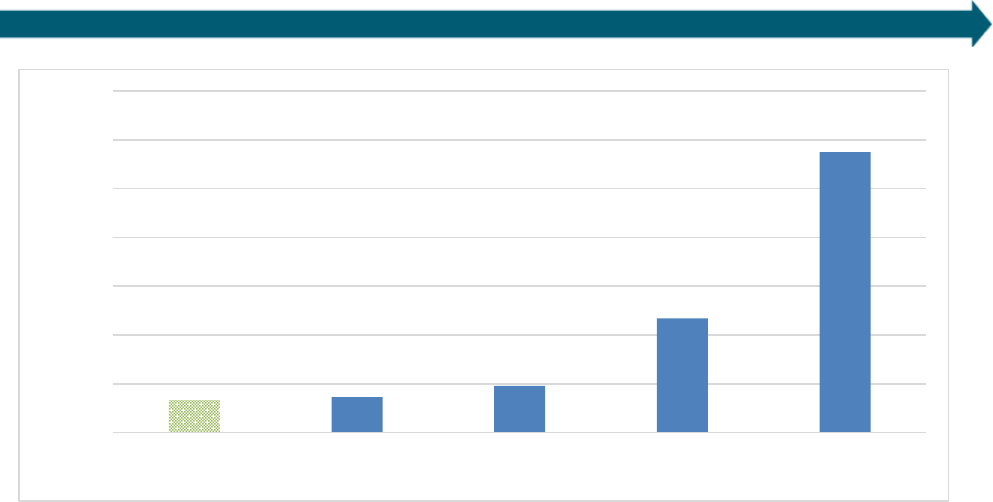
March 2022 www.seeaction.energy.gov 24
Figure 16. Annualized loss rates, energy efficiency loans and comparators
In this comparison, charge-off rates for the pooled energy efficiency portfolios are lower than those for all
comparators including prime auto loans, despite the fact that the energy efficiency loan charge-off rates are gross
rather than net. The pooled energy efficiency loans have a gross annualized charge-off rate of 0.65%, while prime
auto loans show 0.73% and the Fed data on non-credit card consumer loans shows a net annualized charge-off
rate of 0.96%. The fact that the energy efficiency loans show slightly lower annualized losses than auto loans in
Figure 16, but slightly higher losses in Figure 15, likely relates to differences in the construction of the comparators
in terms of their performance over time; overall, loss performance of the studied efficiency loans is very similar to
that of prime auto loans.
5. Conclusions
This report documents and analyzes four large and (in most cases) long-running energy efficiency loan programs to
characterize their financial performance. The energy efficiency loans in this analysis exhibit strong repayment
performance, outperforming other creditworthy unsecured consumer loans and performing comparably to prime
auto loans.
Taking the four studied energy efficiency portfolios together, the overall 30-day delinquency rate of these loans is
1.57%. Losses are highest early in loan lifetimes and decline later, a common finding for consumer loans. The
pooled portfolios lost 2.1% of the principal by year 2, 3.3% by year 4, 4.5% by year 6, and 5.1% by year 8.
Regression analysis on loan-level data shows that credit scores are strongly associated with loan performance, for
both 30-day delinquency and charge-off. Income is also correlated with loan performance; however, this effect is
not as strong as the effect of credit score. Other features of the loans – like loan amounts and interest rates – have
small effects on charge-off rates and no clear relationship with loan delinquency. These results are in line with the
findings of other loan-level analyses of energy efficiency loan and solar PV financing performance (Deason 2015;
Deason, Leventis and Murphy, 2021).
One implication of these regression findings is that borrowers from low-income areas who have strong credit and
pass household-level debt-to-income screens are likely to repay loans or other extended financing at a reasonable
rate. Such borrowers are not uncommon. Lending to low- and moderate-income households requires careful
consideration of factors unique to these borrowers. See Leventis et al. (2017) for discussion of energy efficiency
financing for low- and moderate-income households.
0%
1%
2%
3%
4%
5%
6%
7%
Pooled EE loans, all
programs
Auto loans, prime
only (KBRA)
Non-credit card cons
loans (Fed)
Consumer loans, with
credit (Fed)
Tier 1 consumer loans
(KBRA)
Annualized Gross Loss Rates

March 2022 www.seeaction.energy.gov 25
When pooled across all four studied programs, energy efficiency loans outperform their most logical comparators
– creditworthy unsecured consumer loans – and overall perform comparably to prime auto loans, which are
secured. This is despite the charge-off comparisons between loans analyzed in this report and these other
products that disadvantage the energy efficiency loans in two senses: this analysis does not include data on
recoveries after charge-off, and in some cases the annualization methods employed likely slightly overestimate the
charge-off rates these programs would achieve when more fully seasoned. These findings are the most
comprehensive evidence yet that energy efficiency loans perform strongly relative to other similar forms of
lending.
Our results fall short of proving a relationship between financial performance and either the projects financed by
these programs or the customers of the programs. To do this properly would require loan-level data for the
comparators as well, to adequately control for other potentially relevant differences. While the energy efficiency
loan data are granular, the comparison indices are highly aggregated. Although Berkeley Lab carefully reviewed
and discussed the definitions of the metrics these indices draw on, some inconsistencies in definitions and
reporting surely exist. Some of the indices considered as comparators do not provide any information on the
average creditworthiness of the borrowers; the relatively high credit scores in the energy efficiency programs (or
other factors Berkeley Lab cannot observe in the comparators) may or may not explain some of the differences in
performance between the energy efficiency loans and the comparators.
Regardless of the explanation, the data speak for themselves: the loans made by these four programs, in
aggregate, have performed well. These loans were made by four carefully designed and carefully administered
programs, and one should not assume that other energy efficiency loans would necessarily perform as well if
program design and administration differ. Nevertheless, when considering these programs and other similar
programs, capital providers might wish to take note of this performance. A useful heuristic for capital providers
might be that these energy efficiency loans perform more like prime auto loans than like unsecured consumer
loans. If energy efficiency loans reliably exhibit stronger performance than other similar loans – as these results
suggest – capital providers and lenders should offer better terms (lower interest rates, longer tenors, or both) on
these products as their performance is further proven.
This analysis demonstrates that financial institutions can market efficiency upgrades to their customers and
provide them with the capital they need to make such improvements at low risk, increasing the efficiency of their
homes in the process. Furthermore, our data show that some households from low- and moderate- income areas
take up energy efficiency loans, and that high-credit borrowers in these areas repay financing at a strong rate.
Thus, energy efficiency lending can help support policy goals related to equitable access to capital, such as the
Biden Administration’s Justice 40 goals and Community Reinvestment Act compliance requirements.
6. Areas for future work
This study presents the most comprehensive evidence on energy efficiency loan performance that is publicly
available to date. That said, additional work could advance understanding of energy efficiency loan performance
further. Additional work on loan performance could include:
• Studying additional energy efficiency loan portfolios to expand sample size and test how generalizable the
results of this study are.
• Accessing loan-level data on comparator loans and including those loans in the dataset. This would permit
controlling for factors (for example, credit scores) that may systematically differ between the loans in this
analysis and comparator loans, more directly revealing whether the energy efficiency loans carry a
performance premium.

March 2022 www.seeaction.energy.gov 26
• Adding household incomes, or estimates of same, for additional programs to the data to see if household
income has a notably different relationship with loan performance than census tract metrics. (As
discussed in Section 3.2.3.2, results thus far suggest that this may not yield very different results.)
• Studying whether realized energy savings materially affect loan performance. Deason (2015) found that
projected savings were not a statistically significant predictor of delinquency in early NYSERDA loans.
However, projected savings do not always correspond to actual savings.
Above and beyond loan performance itself, additional research to support potential program administrators
looking to offer or expand residential energy efficiency lending programs could include:
• Assessing the size of the addressable market for these products.
• Considering the most cost-effective way to offer financial support to expand programs offering these
loans, likely through various forms of credit enhancement (such as loan loss reserves, subordinate capital,
or loan guarantees). Zimring et al. (2013) outlines some preliminary considerations in this regard. This
analysis could inform the design of a support facility (for example, a national loan loss reserve or state-
level facility) by leveraging the energy efficiency loan data analyzed here to set performance expectations
for different types of borrowers, thereby helping to size required financial outlays to expand lending.
• Estimating the potential impact of such financial support, or of other types of support to programs, on the
availability and uptake of energy efficiency loan products and on deployment of energy efficiency
measures.
• Identifying programmatic design elements and credit enhancements that might be best able to extend
capital for energy efficiency to markets that are currently underserved by existing financing options. This
effort could help to promote equitable access and tailor suitable loan products (or other financing
products) to underserved households. Leventis et al. (2017) reviews a number of key considerations in
this regard. The analysis in this paper could serve as a starting point for understanding the level of credit
enhancement needed to reach lower-income or low-credit borrowers.

March 2022 www.seeaction.energy.gov 27
References
Deason, Jeff. (2015). The Impact of On-Bill Programs on Loan Performance: Evidence from the Green Jobs, Green
New York Program. International Energy Program Evaluation Conference, 2015.
https://www.iepec.org/wp-
content/uploads/2015/papers/113.pdf
Deason, Jeff, G. Leventis, and S. Murphy. (2021). Performance of solar leasing for low- and middle-income
customers in Connecticut. Prepared for the U.S. Department of Energy and the Clean Energy States Alliance.
https://eta-
publications.lbl.gov/sites/default/files/berkeley_lab_ct_lmi_solar_lease_performance_final_20210423.pdf
Federal Financial Institutions Examination Council (FFIEC). (2014). A Guide to CRA Data Collection and Reporting.
https://www.ffiec.gov/cra/pdf/2013_CRA_Guide.pdf
Leventis, Greg, Chris Kramer, and Lisa C. Schwartz. (2017). Energy Efficiency Financing for Low- and Moderate-
Income Households: Current State of the Market, Issues, and Opportunities.
https://emp.lbl.gov/publications/energy-efficiency-financing-low-and
Li, Wei, L. Goodman. (2016). Comparing Credit Profiles of American Renters and Owners. Urban Institute.
https://www.urban.org/sites/default/files/publication/78591/2000652-Comparing-Credit-Profiles-of-American-
Renters-and-Owners.pdf
Palmer, K., Walls, M. and T. Gerarden. (2012). “Borrowing to Save Energy: An Assessment of Energy-Efficiency
Financing Programs.” Resources for the Future.
https://www.rff.org/publications/reports/borrowing-to-save-
energy-an-assessment-of-energy-efficiency-financing-programs/
State and Local Energy Efficiency Action Network (SEE Action). (2014a). Energy Efficiency Finance Programs: Use-
case Analysis to Define Data Needs and Guidelines. Prepared by: Peter Thompson, Peter Larsen, Chris Kramer, and
Charles Goldman of Lawrence Berkeley National Laboratory.
https://emp.lbl.gov/publications/energy-efficiency-
finance-programs
State and Local Energy Efficiency Action Network (SEE Action). (2014b). Financing Energy Improvements on Utility
Bills: Market Updates and Key Program Design Considerations for Policymakers and Administrators. Prepared by:
Mark Zimring, Greg Leventis, Merrian Borgeson, Peter Thompson, Ian Hoffman and Charles Goldman of Lawrence
Berkeley National Laboratory. https://eta.lbl.gov/publications/financing-energy-improvements-utility
TransUnion. (2020). “April 2020 Monthly Industry Snapshot.” https://content.transunion.com/v/monthly-industry-
snapshot-april-final?utmsource=press-release
Zimring, Mark, Merrian Borgeson, Annka Todd, and Chuck Goldman. (2013). Getting the Biggest Bang for the Buck:
Exploring the Rationales and Design Options for Energy Efficiency Financing Programs. Lawrence Berkeley National
Laboratory. https://eta-publications.lbl.gov/sites/default/files/lbnl-6524e.pdf

March 2022 www.seeaction.energy.gov
Appendix A: Regression results
The table below summarizes the regression results used in Section 3.2.3. The average marginal effects for credit
score, seasoning, interest, and principal amount all measure the change in likelihood of the outcome variable (e.g.,
charge-off) for a unit increase in each variable. For categorical variables like AMI band or program, the average
marginal effects represent the change in likelihood for some outcome relative to some base case. For the four AMI
bands in the table, the base case is the 0-60% AMI band. For program comparisons, Michigan Saves serves as the
base case.
Table A-1. Regression output for all loan portfolios combined (n=51,041)
30-
120 Day Delinquency Charge-off
Dependent Variable
Average
Marginal
Effects
Standard
Error
P Value
Average
Marginal
Effects
Standard
Error
P Value
Credit Score
-1.06E-04
8.09E-06
2.06E-39
-5.81E-04
1.76E-05
8.82E-240
Seasoning (Days)
-3.12E-06
5.77E-07
6.20E-08
2.07E-05
1.01E-06
4.71E-93
Interest Rate
-5.87E-02
3.36E-02
8.00E-02
2.29E-01
6.45E-02
3.75E-04
Principal Amount ($)
4.29E-08
6.72E-08
5.23E-01
4.61E-07
1.61E-07
4.23E-03
Smart-E
7.85E-03
1.73E-03
6.04E-06
-1.23E-02
6.01E-03
4.00E-02
NYSERDA On-Bill
Recovery
1.91E-02
1.65E-03
2.88E-31
6.09E-03
3.84E-03
1.13E-01
NYSERDA Smart-
Energy
3.54E-03
1.37E-03
9.50E-03
1.37E-02
2.63E-03
2.13E-07
Keystone
5.00E-04
1.84E-03
7.86E-01
2.06E-03
2.79E-03
4.61E-01
Table A-2. Regression output for all loan portfolios with income (n+36,288)
30-
120 Day Delinquency Charge-off
Dependent Variable
Average
Marginal
Effects
Standard
Error
P Value
Average
Marginal
Effects
Standard
Error
P Value
Credit Score
-1.281E-
04
1.054E-05
5.828E-34
-5.264E-
04
1.919E-05
1.106E-
165
Seasoning (Days)
-4.178E-
06
8.405E-07
6.669E-07
1.956E-05
1.202E-06
1.479E-59
Interest Rate
-5.838E-
02
5.209E-02
2.624E-01
3.106E-01
8.606E-02
3.068E-04
Principal Amount ($)
8.638E-08
8.786E-08
3.255E-01
4.376E-07
1.587E-07
5.820E-03
60%-80% + AMI
7.537E-04
1.579E-03
6.332E-01
6.521E-04
2.667E-03
8.069E-01
80%-100% + AMI
-1.911E-
04
1.505E-03
8.990E-01
-5.883E-
03
2.634E-03
2.553E-02
A-1

March 2022 www.seeaction.energy.gov
100%-120% + AMI
-4.987E-
03
2.061E-03
1.553E-02
-8.617E-
03
3.380E-03
1.080E-02
120%+ AMI
-5.030E-
03
2.288E-03
2.788E-02
-1.985E-
02
4.309E-03
4.075E-06
Smart-E
1.037E-02
2.272E-03
5.065E-06
-9.057E-
03
5.632E-03
1.078E-01
NYSERDA On-Bill
Recovery
2.469E-02
2.175E-03
7.198E-30
6.040E-03
3.826E-03
1.145E-01
NYSERDA Smart-
Energy
4.453E-03
1.783E-03
1.251E-02
1.200E-02
2.740E-03
1.198E-05
Table A-3. Regression output for Michigan Saves (n=14,905)
30-120 Day Delinquency Charge-off
Dependent Variable
Average
Marginal
Effects
Standard
Error
P-Value
Average
Marginal
Effects
Standard
Error
P-Value
Credit Score
-7.445E-
05
1.460E-05
0.000E+00
-4.000E-
04
3.280E-05
0.000E+0
0
Seasoning (Days)
-1.933E-
06
7.730E-07
1.200E-02
2.092E-05
1.580E-06
0.000E+0
0
Interest Rate
-5.620E-
02
4.400E-02
1.990E-01
1.443E-01
7.400E-02
5.200E-02
Principal Amount ($)
-3.665E-
08
1.010E-07
7.160E-01
6.573E-07
1.930E-07
1.000E-03
60%-80% + AMI
-2.400E-
03
2.000E-03
1.820E-01
-1.400E-
03
4.000E-03
7.100E-01
80%-100% + AMI
-1.500E-
03
2.000E-03
3.750E-01
-1.130E-
02
4.000E-03
4.000E-03
100%-120% + AMI
-4.100E-
03
2.000E-03
6.000E-02
-9.000E-
03
4.000E-03
4.400E-02
120%+ AMI
-6.100E-
03
3.000E-03
2.500E-02
-2.450E-
02
6.000E-03
0.000E+0
0
Table A-4. Regression output for CT Smart-E (n=3,166)
30-120 Day Delinquency Charge-off
Dependent Variable
Average
Marginal
Effects
Standard
Error
P-Value
Average
Marginal
Effects
Standard
Error
P-Value
Credit Score
-2.133E-04
4.894E-
05
1.306E-
05
-2.320E-
04
4.974E-
05
3.093E-
06
Seasoning (Days)
-2.126E-06
5.097E-
06
6.767E-
01
1.337E-
05
3.700E-
06
3.015E-
04
Interest Rate
2.313E-02
1.138E-
01
8.389E-
01
4.486E-
02
9.989E-
02
6.534E-
01
A-2

March 2022 www.seeaction.energy.gov
Principal Amount ($)
5.859E-07
2.801E-
07
3.647E-
02
1.406E-
07
2.904E-
07
6.282E-
01
60%-80% + AMI
1.413E-02
9.366E-
03
1.313E-
01
-3.760E-
03
6.567E-
03
5.670E-
01
80%-100% + AMI
1.751E-02
8.914E-
03
4.949E-
02
5.252E-
03
5.460E-
03
3.361E-
01
100%-120% + AMI
1.052E-02
9.760E-
03
2.810E-
01
-4.285E-
03
6.877E-
03
5.332E-
01
120%+ AMI
1.103E-02
9.835E-
03
2.621E-
01
-1.418E-
02
1.014E-
02
1.622E-
01
Ta
ble A-5. Regression output for Keystone HELP (n=14,753)
30-120 Day Delinquency Charge-off
Dependent Variable
Average
Marginal
Effects
Standard
Error
P-Value
Average
Marginal
Effects
Standard
Error
P-Value
Credit Score
-5.646E-05
1.320E-
05
1.903E-
05
-7.247E-
04
4.099E-
05
5.766E-
70
Seasoning (Days)
-8.444E-07
4.786E-
07
7.767E-
02
2.240E-
05
2.110E-
06
2.420E-
26
Interest Rate
-3.102E-02
2.279E-
02
1.736E-
01
2.803E-
01
1.146E-
01
1.442E-
02
Principal Amount ($)
7.119E-08
1.331E-
07
5.927E-
01
1.143E-
06
5.896E-
07
5.261E-
02
Table 5. Regression output for NYSERDA Smart Energy (n=14,176)
30-120 Day Delinquency Charge-off
Dependent Variable
Average
Marginal
Effects
Standard
Error
P-Value
Average
Margina
l Effects
Standard
Error
P-Value
Credit Score
-1.236E-04
1.544E-
05
1.205E-
15
-6.703E-
04
3.265E-
05
1.114E-93
Seasoning (Days)
-3.555E-06
1.122E-
06
1.535E-
03
2.134E-
05
2.289E-
06
1.132E-20
Interest Rate
-9.784E-02
9.953E-
02
3.256E-
01
3.829E-
02
2.536E-
01
8.800E-01
Principal Amount ($)
1.615E-07
1.484E-
07
2.764E-
01
-1.833E-
07
3.359E-
07
5.853E-01
A-3

March 2022 www.seeaction.energy.gov
Debt-to-Income Ratio (DTI)
1.157E-03
7.455E-
04
1.205E-
01
1.781E-
03
3.402E-
03
6.006E-01
Table 6. Regression output for NYSERDA On-Bill Recovery (n=3,849)
30-120 Day Delinquency Charge-off
Dependent Variable
Average
Marginal
Effects
Standard
Error
P-Value
Average
Marginal
Effects
Standard
Error
P-Value
Credit Score
-2.773E-04
5.653E-
05
9.335E-
07
-5.525E-
04
5.872E-
05
4.939E-21
Seasoning (Days)
-1.094E-05
5.773E-
06
5.821E-
02
-2.164E-
07
6.048E-
06
9.715E-01
Interest Rate
-1.994E-01
6.060E-
01
7.421E-
01
-4.326E-
01
7.105E-
01
5.426E-01
Principal Amount ($)
-1.972E-07
4.661E-
07
6.723E-
01
1.414E-
06
4.400E-
07
1.313E-03
Debt-to-Income Ratio (DTI)
4.248E-03
1.652E-
02
7.971E-
01
-1.087E-
04
1.669E-
02
9.948E-01
A-4
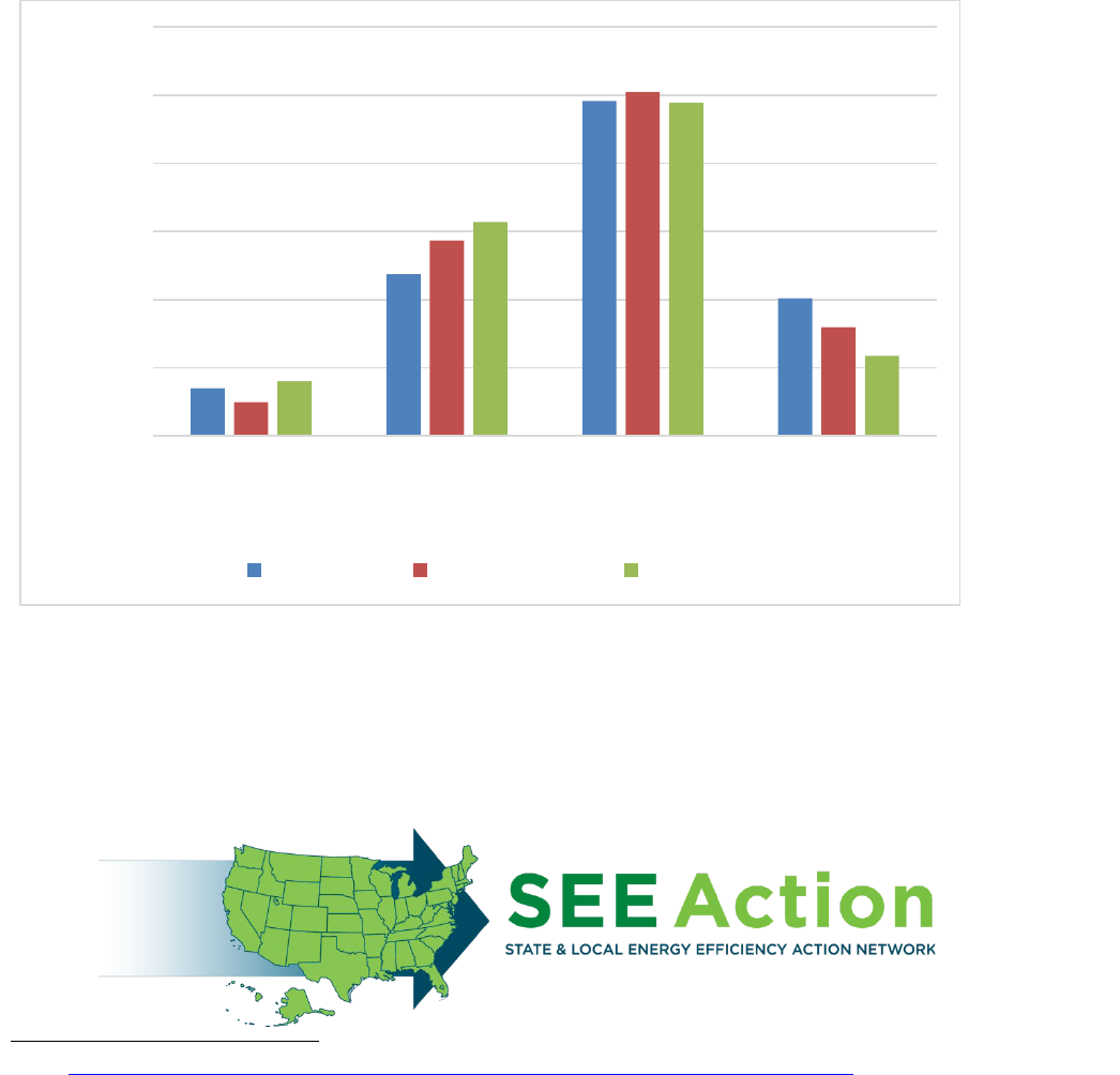
March 2022 www.seeaction.energy.gov
Appendix B: Participation by Community Reinvestment Act income bin
The Federal Reserve Board, the Federal Deposit Insurance Corporation, and the Office of the Comptroller of the
Currency (OCC) enforce regulations to implement the Community Reinvestment Act (CRA) of 1977. The CRA
“encourages insured depository institutions to help meet the credit needs of the communities in which they are
chartered” (FFIEC, 2012), including low- and moderate-income neighborhoods. For purposes of the CRA, the OCC
defines low-income as household income that is less than 50% of AMI, moderate-income is 50% to 80% of AMI,
middle-income is 80% to 120% of AMI, and upper-income is 120% or more of AMI.
21
Figure 17 shows participation
in the studied programs by those CRA bins.
Figure 17. Participation by CRA income bin
21
See https://www.federalregister.gov/documents/2020/06/05/2020-11220/community-reinvestment-act-regulations.
0%
10%
20%
30%
40%
50%
60%
<50% 50%-80% 80%-120% >120%
% of loans
CRA AMI bins
CT Smart-E Michigan Saves NYSERDA
This document was developed as a product of the State and Local Energy Efficiency Action Network (SEE Action), facilitated by the U.S.
Department of Energy/U.S. Environmental Protection Agency. Content does not imply an endorsement by the individuals or organizations that
are part of SEE Action working groups, or reflect the views, policies, or otherwise of the federal government.
B-1
